SUSY vs. The Machines

Article title: Bayesian Neural Networks for Fast SUSY Predictions

Authors: B. S. Kronheim, M. P. Kuchera, H. B. Prosper, A. Karbo

Reference: https://arxiv.org/abs/2007.04506

It has been a while since we have graced these parts with the sounds of the attractive yet elusive superhero named SUSY. With such an arduous history of experimental effort, supersymmetry still remains unseen by the eyes of even the most powerful colliders. Though in the meantime, phenomenologists and theorists continue to navigate the vast landscape of model parameters with hopes of narrowing in on the most intriguing predictions – even connecting dark matter into the whole mess.

How vast you may ask? Well the ‘vanilla’ scenario, known as the Minimal Supersymmetric Standard Model (MSSM) – containing partner particles for each of those of the Standard Model – is chock-full of over 100 free parameters. This makes rigorous explorations of the parameter space not only challenging to interpret, but also computationally expensive. In fact, the standard practice is to confine oneself to a subset of the parameter space, using suitable justifications, and go ahead to predict useful experimental observables like collider production rates or particle masses. One of these popular motivations is known as the phenoneological MSSM (pMSSM), which reduces the huge parameter area to just less than 20 by assuming the absence of things like SUSY-driven CP-violation, flavour changing neutral currents (FCNCs) and differences between first and second generation SUSY particles. With this in the toolbox, computations become comparatively more feasible, with just enough complexity to make solid but interesting predictions.

But even coming from personal experience, these spaces can still be typically be rather tedious to work through – especially since many parameter selections are theoretically nonviable and/or in disagreement with previously well-established experimental observables, like the mass of the Higgs Boson. Maybe there is a faster way?

Machine learning has shared a successful history with a lot of high-energy physics applications, particularly those with complex dynamics like SUSY. One particularly useful application, at which machine learning is very accomplished at, is classification of points as excluded or not excluded based on searches at the LHC by ATLAS and CMS.

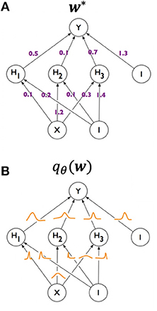
In the considered paper, a special type of Neural Network (NN) known as a Bayesian Neural Network (BNN) is used, which notably rely on probablistic certainty of classification rather than simply classifying a result as one thing or the other.

Figure 1: Your standard Neural Network (NN) shown in A has a single weight for each of its neuron connections (just represented by a number), learned from the training set. However, a Bayesian Neural Network (BNN) represented in B instead has a posterior distribution for each weight. When trained, it takes a prior distribution and applies Bayesian methods to obtain a posterior distribution. Taken from https://doi.org/10.3389/fninf.2019.00067.

In a typical NN there is a space of adjustable parameters (often called “features”) and a list of “targets” for the model to learn classification from. In this particular case, the model parameters are of course the features to learn from – these mainly include mass parameters for the different superparticles in the spectrum. These are mapped to three different predictions or targets that can be computed from these parameters:

The mass of the lightest, neutral Higgs Boson (the 125 GeV one)
The cross sections of processes involving the superpartners to the elecroweak guage bosons (typically called the neutralinos and charginos – I will let you figure out which ones are the charged and neutral ones)
Whether the point is actually valid or not (or maybe theoretically consistent is a better way to put it).

Of course there is an entire suite of programs designed to carry out these calculations, which are usually done point by point in the parameter space of the pMSSM, and hence these would be used to construct the training data sets for the algorithm to learn from – one data set for each of the predictions listed above.

But how do we know our model is trained properly once we have finished the learning process? There are a number of metrics that are very commonly used to determine whether a machine learning algorithm can correctly classify the results of a set of parameter points. The following table sums up the four different types of classifications that could be made on a set of data.

Table 1: Classifications for data given the predicted and actual results.

The typical measures employed using this table are the precision, recall and F1 score which are in practice readily defined as:

$P = \frac{TP}{TP+FP}, \quad R = \frac{TP}{TP+FN}, \quad F_1 = 2\frac{P \cdot R}{P+R}.$

In predicting the validity of points, the recall especially will tell us the fraction of valid points that will be correctly identified by the algorithm. For example, the metrics for this validity data set are shown in Table 2.

Table 2: Metrics for point validity data set. A point is valid from the classifier if it exceeds a cutoff of 0.5 in the first row, with a more relaxed 3 standard deviations in the second.

With a higher Recall but lower precision for the 3 standard deviation cutoff it is clear that points with a larger uncertainty will be classified as valid in this case. Such a scenario would be useful in calculating further properties like the mass spectrum, but not neccesarily as the best classifier.

Similarly with the data set used to compute cross sections, the standard deviation can be used for points where the predictions are quite uncertain. On average their calculations revealed just over 3% percent error with the actual value of the cross section. Not to be outdone, in calculating the Higgs boson mass, within 2 GeV deviation of 125 GeV, the precision of the BNN was found to be 0.926 with a recall of 0.997, showing that very few parameter points that are actually conistent with the light neutral Higgs will actually be removed.

In the end, our whole purpose was to provide reliable SUSY predictions at a fraction of the time. It is well known that NNs provide relatively fast calculation, especially when utilizing powerful hardware, and in this case could acheive up to over 16 million times faster in computing a single point than standard SUSY software! Finally, it is worth to note that neural networks are highly scalable and so predictions from the 19-dimensional pMSSM are but one of the possibilities for NNs in calculating SUSY observables.

Futher Reading

[1] Bayesian Neural Networks and how they differ from traditional NNs: https://towardsdatascience.com/making-your-neural-network-say-i-dont-know-bayesian-nns-using-pyro-and-pytorch-b1c24e6ab8cd

[2] More on machine learning and A.I. and its application to SUSY: https://arxiv.org/abs/1605.02797

Print Friendly