While searching for new Higgs bosons the CMS experiment at the Large Hadron Collider (LHC) may have just found a surprise. They have observed an excess of events that look to be a new particle, and are reporting high statistical evidence for their claim. The only question is what exactly is this new particle?
The search was initially designed to look for new, heavier, versions of the Higgs boson decaying to a top quark and an anti-top quark. Its well known that the Higgs boson of the Standard Model, discovered jointly by ATLAS and CMS in 2012, underlies the mechanism which gives all fundamental particles their masses. The Higgs boson itself interacts with particles in proportion to their mass, preferring heavier particles over lighter ones. It therefore interacts the most strongly with the heaviest known fundamental particle, the top quark, which has a mass of ~173 GeV. The Higgs boson itself only has a bass of 125 GeV, meaning conservation of energy dictates it can’t decay into a top quark-antiquark pair.
However many theories of physics beyond the the Standard Model predict additional Higgs bosons, heavier cousins of the current one. If these new heavy Higgs bosons had a mass larger than 350 GeV, they would likely decay to a top quark-antiquark pair quite often. CMS therefore was analyzed its data searching for this signature, hoping to find signs of a new Higgs boson. To do so, they had scrutinize very carefully the known production of top quark-antiquark pairs, which are produced copiously at the LHC from other processes. If a new particle was being produced and decaying to top quarks, the mass of the new particle would give the top quarks a characteristic energy. One key sign of a new particle would therefore be an excess of top quark-antiquark events at a particular energy, corresponding to the mass of the new particle.
When CMS scrutinized their data looking for such an excess they found one. But curiously right ~350 GeV, the minimum energy required to produce the top quark-antiquark pair. It would be quite the coincidence for a new particle to show up right at this minimum threshold, which made CMS consider alternative possibilities.
A comparison of the observed CMS data and their estimate of backgrounds as a function of the invariant mass of the top quark antiquark system. CMS observes an excess of events at ~350 GeV, which is well fit with a toponium model (red line).
One unorthodox explanation that seems to fit the bill is ‘toponium’, a short lived bound state of the top quark-antiquark pair is being formed. Toponium would be the heaviest version of ‘quarkonia’ we have seen, bound states of quark antiquark pairs that form bound states similar to atoms. We have observed and measured quarkonia states of the other quarks for decades, however it was long thought that the top quark, whose large mass causes it to decay in just 10^(-25) seconds, would decay too quickly to create observable bound state effects at a hadron collider. Toponium production would happen most often if the top quarks were produced just at the energy threshold, such that they don’t any extra energy. These low energy top quarks would spend more time close to each other than normal, rather than immediately flying away, so they could have time to briefly form a toponium state before decaying. However, once small hints of intriguing excesses started appearing in LHC analyses, updated calculations in the last few years suggested that perhaps such an effect could be observable.
These calculations are approximate, and more work is still being done to refine them. But the preliminary predictions they give for the properties of toponium seem to match well with what CMS is seeing, both in terms of the rate of toponium production and the quantum properties of the toponium state (spin and parity).
Still CMS is being cautious before claiming a discovery of toponium. They claim observation of an ‘excess at the top quark pair production threshold’ which is consistent with toponium. However given the limited present data and incomplete theoretical models of toponium, they cannot rule out that the excess they are seeing is coming from a new Higgs-like particle.
CMS measurement tries to disentangle the quantum properties of the observed excess. The x-axis shows the estimated rate of production a ‘pseudoscalar’ particle producing the excess. The y-axis shows a similar estimate for a ‘scalar’ particle. The allowed region for the scalar still includes zero, while the zero pseudoscalar hypothesis is clearly excluded at larger than 5 standard deviations.
Further work will be needed to develop improved theoretical models of toponium, and detailed studies from CMS assessing the properties of their observed excess. The excess will also need confirmation from CMS’s rival LHC experiment, ATLAS, to ensure it has not merely made a mistake in its analysis.
However, the smart money would say this very likely looks like toponium. Which, while not signaling the long sought overthrow of the standard model, would be an unexpected and cool surprise from the LHC. Understanding the properties of this previously-thought-impossible quasiparticle will spawn much fruitful research in the years to come. Physicists love a surprise!
Discloure: The author is a member of the CMS collaboration but did not directly work on this analysis
Erratum 4/15/2025 : The article was updated to clarify that in the theory literature prior to the LHC toponium was thought possible to form, just that it was thought to be too small an effect to be observable. The article previously incorrectly stated it had been previously thought impossible to form
This is the second part of our coverage of the P5 report and its implications for particle physics. To read the first part, click here
One of the thorniest questions in particle physics is ‘What comes after the LHC?’. This was one of the areas people were most uncertain what the P5 report would say. Globally, the field is trying to decide what to do once the LHC winds down in ~2040 While the LHC is scheduled to get an upgrade in the latter half of the decade and run until the end of the 2030’s, the field must start planning now for what comes next. For better or worse, big smash-y things seem to capture a lot of public interest, so the debate over what large collider project to build has gotten heated. Even Elon Musk is tweeting (X-ing?) memes about it.
Famously, the US’s last large accelerator project, the Superconducting Super Collider (SSC), was cancelled in the ’90s partway through its construction. The LHC’s construction itself often faced perilous funding situations, and required a CERN to make the unprecedented move of taking a loan to pay for its construction. So no one takes for granted that future large collider projects will ultimately come to fruition.
Desert or Discovery?
When debating what comes next, dashed hopes of LHC discoveries are top of mind. The LHC experiments were primarily designed to search for the Higgs boson, which they successfully found in 2012. However, many had predicted (perhaps over-confidently) it would also discover a slew of other particles, like those from supersymmetry or those heralding extra-dimensions of spacetime. These predictions stemmed from a favored principle of nature called ‘naturalness’ which argued additional particles nearby in energy to the Higgs were needed to keep its mass at a reasonable value. While there is still much LHC data to analyze, many searches for these particles have been performed so far and no signs of these particles have been seen.
These null results led to some soul-searching within particle physics. The motivations behind the ‘naturalness’ principle that said the Higgs had to be accompanied by other particles has been questioned within the field, and in New York Times op-eds.
No one questions that deep mysteries like the origins of dark matter, matter anti-matter asymmetry, and neutrino masses, remain. But with the Higgs filling in the last piece of the Standard Model, some worry that answers to these questions in the form of new particles may only exist at energy scales entirely out of the reach of human technology. If true, future colliders would have no hope of
A diagram of the particles of the Standard Model laid out as a function of energy. The LHC and other experiments have probed up to around 10^3 GeV, and found all the particles of the Standard Model. Some worry new particles may only exist at the extremely high energies of the Planck or GUT energy scales. This would imply a large large ‘desert’ in energy, many orders of magnitude in which no new particles exist. Figure adapted from here
The situation being faced now is qualitatively different than the pre-LHC era. Prior to the LHC turning on, ‘no lose theorems’, based on the mathematical consistency of the Standard Model, meant that it had to discover the Higgs or some other new particle like it. This made the justification for its construction as bullet-proof as one can get in science; a guaranteed Nobel prize discovery. But now with the last piece of the Standard Model filled in, there are no more free wins; guarantees of the Standard Model’s breakdown don’t occur until energy scales we would need solar-system sized colliders to probe. Now, like all other fields of science, we cannot predict what discoveries we may find with future collider experiments.
Still, optimists hope, and have their reasons to believe, that nature may not be so unkind as to hide its secrets behind walls so far outside our ability to climb. There are compelling models of dark matter that live just outside the energy reach of the LHC, and predict rates too low for direct detection experiments, but would be definitely discovered or ruled out by high energy colliders. The nature of the ‘phase transition’ that occurred in the very early universe, which may explain the prevalence of matter over anti-matter, can also be answered. There are also a slew ofexperimental ‘hints‘, all of which have significant question marks, but could point to new particles within the reach of a future collider.
Many also just advocate for building a future machine to study nature itself, with less emphasis on discovering new particles. They argue that even if we only further confirm the Standard Model, it is a worthwhile endeavor. Though we calculate Standard Model predictions for high energies, unless they are tested in a future collider we will not ‘know’ how if nature actually works like this until we test it in those regimes. They argue this is a fundamental part of the scientific process, and should not be abandoned so easily. Chief among the untested predictions are those surrounding the Higgs boson. The Higgs is a central somewhat mysterious piece of the Standard Model but is difficult to measure precisely in the noisy environment of the LHC. Future colliders would allow us to study it with much better precision, and verify whether it behaves as the Standard Model predicts or not.
Projects
These theoretical debates directly inform what colliders are being proposed and what their scientific case is.
Many are advocating for a “Higgs factory”, a collider of based on clean electron-positron collisions that could be used to study the Higgs in much more detail than the messy proton collisions of the LHC. Such a machine would be sensitive to subtle deviations of Higgs behavior from Standard Model predictions. Such deviations could come from the quantum effects of heavy, yet-undiscovered particles interacting with the Higgs. However, to determine what particles are causing those deviations, its likely one would need a new ‘discovery’ machine which has high enough energy to produce them.
Among the Higgs factory options are the International Linear Collider, a proposed 20km linear machine which would be hosted in Japan. ILC designs have been ‘ready to go’ for the last 10 years but the Japanese government has repeated waffled on whether to approve the project. Sitting in limbo for this long has led to many being pessimistic about the projects future, but certainly many in the global community would be ecstatic to work on such a machine if it was approved.
Designs for the ILC have been ready for nearly a decade, but its unclear if it will receive the greenlight from the Japanese government. Image source
Alternatively, some in the US have proposed building a linear collider based on a ‘cool copper’ cavities (C3) rather than the standard super conducting ones. These copper cavities can achieve more acceleration per meter than the standard super conducting ones, meaning a linear Higgs factory could be constructed with a reduced 8km footprint. A more compact design can significantly cut down on infrastructure costs that governments usually don’t like to use their science funding on. Advocates had proposed it as a cost-effective Higgs factory option, whose small footprint means it could potentially hosted in the US.
The Future-Circular-Collider (FCC), CERN’s successor to the LHC, would kill both birds with one extremely long stone. Similar to the progression from LEP to the LHC, this new proposed 90km collider would run as Higgs factory using electron-positron collisions starting in 2045 before eventually switching to a ~90 TeV proton-proton collider starting in ~2075.
Designs for the massive 90km FCC ring surrounding Geneva
Such a machine would undoubtably answer many of the important questions in particle physics, however many have concerns about the huge infrastructure costs needed to dig such a massive tunnel and the extremely long timescale before direct discoveries could be made. Most of the current field would not be around 50 years from now to see what such a machine finds. The Future-Circular-Collider (FCC), CERN’s successor to the LHC, would kill both birds with one extremely long stone. Similar to the progression from LEP to the LHC, this new proposed 90km collider would run as Higgs factory using electron-positron collisions starting in 2045 before eventually switching to a ~90 TeV proton-proton collider starting in ~2075. Such a machine would undoubtably answer many of the important questions in particle physics, however many have concerns about the extremely long timescale before direct discoveries could be made. Most of the current field would not be around 50 years from now to see what such a machine finds. The FCC is also facing competition as Chinese physicists have proposed a very similar design (CEPC) which could potentially start construction much earlier.
During the snowmass process many in the US starting pushing for an ambitious alternative. They advocated a new type of machine that collides muons, the heavier cousin of electrons. A muon collider could reach the high energies of a discovery machine while also maintaining a clean environment that Higgs measurements can be performed in. However, muons are unstable, and collecting enough of them into formation to form a beam before they decay is a difficult task which has not been done before. The group of dedicated enthusiasts designed t-shirts and Twitter memes to capture the excitement of the community. While everyone agrees such a machine would be amazing, the key technologies necessary for such a collider are less developed than those of electron-positron and proton colliders. However, if the necessary technological hurdles could be overcome, such a machine could turn on decades before the planned proton-proton run of the FCC. It can also presents a much more compact design, at only 10km circumfrence, roughly three times smaller than the LHC. Advocates are particularly excited that this would allow it to be built within the site of Fermilab, the US’s flagship particle physics lab, which would represent a return to collider prominence for the US.
A proposed design for a muon collider. It relies on ambitious new technologies, but could potentially deliver similar physics to the FCC decades sooner and with a ten times smaller footprint. Source
Deliberation & Decision
This plethora of collider options, each coming with a very different vision of the field in 25 years time led to many contentious debates in the community. The extremely long timescales of these projects led to discussions of human lifespans, mortality and legacy being much more being much more prominent than usual scientific discourse.
Ultimately the P5 recommendation walked a fine line through these issues. Their most definitive decision was to recommend against a Higgs factor being hosted in the US, a significant blow to C3 advocates. The panel did recommend US support for any international Higgs factories which come to fruition, at a level ‘commensurate’ with US support for the LHC. What exactly ‘comensurate’ means in this context I’m sure will be debated in the coming years.
However, the big story to many was the panel’s endorsement of the muon collider’s vision. While recognizing the scientific hurdles that would need to be overcome, they called the possibility of muon collider hosted in the US a scientific ‘muon shot‘, that would reap huge gains. They therefore recommended funding for R&D towards they key technological hurdles that need to be addressed.
Because the situation is unclear on both the muon front and international Higgs factory plans, they recommended a follow up panel to convene later this decade when key aspects have clarified. While nothing was decided, many in the muon collider community took the report as a huge positive sign. While just a few years ago many dismissed talk of such a collider as fantastical, now a real path towards its construction has been laid down.
Hitoshi Murayama, chair of the P5 committee, cuts into a ‘Shoot for the Muon’ cake next to a smiling Lia Merminga, the director of Fermilab. Source
While the P5 report is only one step along the path to a future collider, it was an important one. Eyes will now turn towards reports from the different collider advocates. CERN’s FCC ‘feasibility study’, updates around the CEPC and, the International Muon Collider Collaboration detailed design report are all expected in the next few years. These reports will set up the showdown later this decade where concrete funding decisions will be made.
For those interested the full report as well as executive summaries of different areas can be found on the P5 website. Members of the US particle physics community are also encouraged to sign the petition endorsing the recommendations here.
When students first learn quantum field theory, the mathematical language the underpins the behavior of elementary particles, they start with the simplest possible interaction you can write down : a particle with no spin and no charge scattering off another copy of itself. One then eventually moves on to the more complicated interactions that describe the behavior of fundamental particles of the Standard Model. They may quickly forget this simplified interaction as a unrealistic toy example, greatly simplified compared to the complexity the real world. Though most interactions that underpin particle physics are indeed quite a bit more complicated, nature does hold a special place for simplicity. This barebones interaction is predicted to occur in exactly one scenario : a Higgs boson scattering off itself. And one of the next big targets for particle physics is to try and observe it.
A Feynman diagram of the simplest possible interaction in quantum field theory, a spin-zero particle interacting with itself.
The Higgs is the only particle without spin in the Standard Model, and the only one that doesn’t carry any type of charge. So even though particles such as gluons can interact with other gluons, its never two of the same kind of gluons (the two interacting gluons will always carry different color charges). The Higgs is the only one that can have this ‘simplest’ form of self-interaction. Prominent theorist Nima Arkani-Hamed has said that the thought of observing this “simplest possible interaction in nature gives [him] goosebumps“.
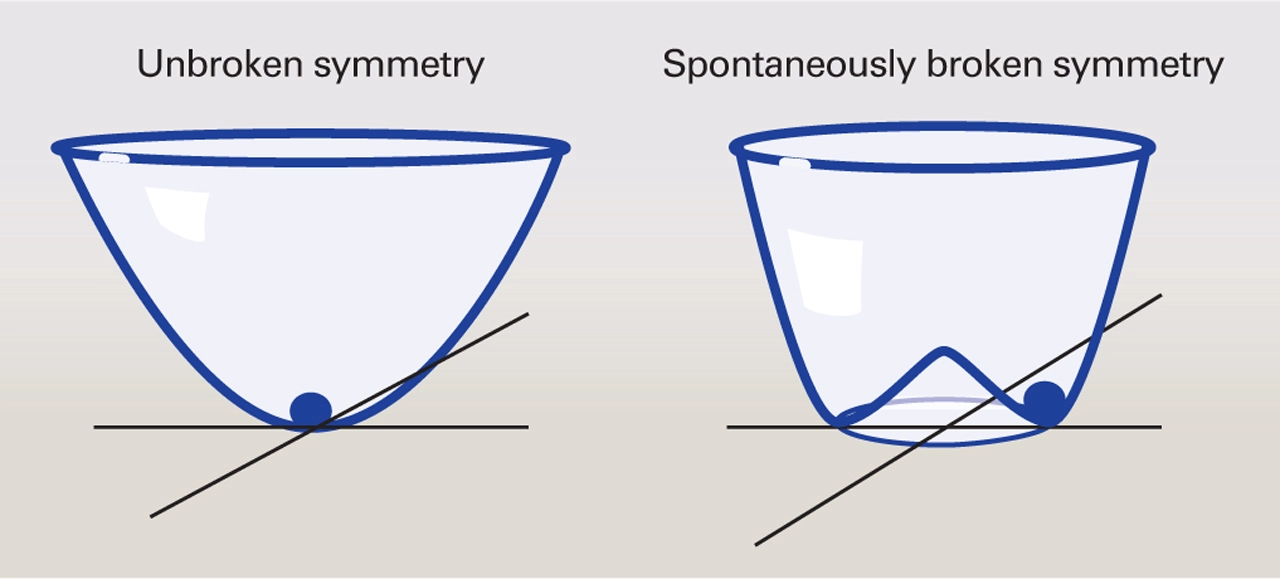
But more than being interesting for its simplicity, this self-interaction of the Higgs underlies a crucial piece of the Standard Model: the story of how particles got their mass. The Standard Model tells us that the reason all fundamental particles have mass is their interaction with the Higgs field. Every particle’s mass is proportional to the strength of the Higgs field. The fact that particles have any mass at all is tied to the fact that the lowest energy state of the Higgs field is at a non-zero value. According to the Standard Model, early in the universe’s history when the temperature were much higher, the Higgs potential had a different shape, with its lowest energy state at field value of zero. At this point all the particles we know about were massless. As the universe cooled the shape of the Higgs potential morphed into a ‘wine bottle’ shape, and the Higgs field moved into the new minimum at non-zero value where it sits today. The symmetry of the initial state, in which the Higgs was at the center of its potential, was ‘spontaneously broken’ as its new minimum, at a location away from the center, breaks the rotation symmetry of the potential. Spontaneous symmetry breaking is a very deep theoretical idea that shows up not just in particle physics but in exotic phases of matter as well (eg superconductors).
A diagram showing the ‘unbroken’ Higgs potential in the very early universe (left) and the ‘wine bottle’ shape it has today (right). When the Higgs at the center of its potential it has a rotational symmetry, there are no preferred directions. But once it finds it new minimum that symmetry is broken. The Higgs now sits at a particular field value away from the center and a preferred direction exists in the system.
This fantastical story of how particle’s gained their masses, one of the crown jewels of the Standard Model, has not yet been confirmed experimentally. So far we have studied the Higgs’s interactions with other particles, and started to confirm the story that it couples to particles in proportion to their mass. But to confirm this story of symmetry breaking we will to need to study the shape of the Higgs’s potential, which we can probe only through its self-interactions. Many theories of physics beyond the Standard Model, particularly those that attempt explain how the universe ended up with so much matter and very little anti-matter, predict modifications to the shape of this potential, further strengthening the importance of this measurement.
Unfortunately observing the Higgs interacting with itself and thus measuring the shape of its potential will be no easy feat. The key way to observe the Higgs’s self-interaction is to look for a single Higgs boson splitting into two. Unfortunately in the Standard Model additional processes that can produce two Higgs bosons quantum mechanically interfere with the Higgs self interaction process which produces two Higgs bosons, leading to a reduced production rate. It is expected that a Higgs boson scattering off itself occurs around 1000 times less often than the already rare processes which produce a single Higgs boson. A few years ago it was projected that by the end of the LHC’s run (with 20 times more data collected than is available today), we may barely be able to observe the Higgs’s self-interaction by combining data from both the major experiments at the LHC (ATLAS and CMS).
Fortunately, thanks to sophisticated new data analysis techniques, LHC experimentalists are currently significantly outpacing the projected sensitivity. In particular, powerful new machine learning methods have allowed physicists to cut away background events mimicking the di-Higgs signal much more than was previously thought possible. Because each of the two Higgs bosons can decay in a variety of ways, the best sensitivity will be obtained by combining multiple different ‘channels’ targeting different decay modes. It is therefore going to take a village of experimentalists each working hard to improve the sensitivity in various different channels to produce the final measurement. However with the current data set, the sensitivity is still a factor of a few away from the Standard Model prediction. Any signs of this process are only expected to come after the LHC gets an upgrade to its collision rate a few years from now.
Current experimental limits on the simultaneous production of two Higgs bosons, a process sensitive to the Higgs’s self-interaction, from ATLAS (left) and CMS (right). The predicted rate from the Standard Model is shown in red in each plot while the current sensitivity is shown with the black lines. This process is searched for in a variety of different decay modes of the Higgs (various rows on each plot). The combined sensitivity across all decay modes for each experiment allows them currently to rule out the production of two Higgs bosons at 3-4 times the rate predicted by the Standard Model. With more data collected both experiments will gain sensitivity to the range predicted by the Standard Model.
While experimentalists will work as hard as they can to study this process at the LHC, to perform a precision measurement of it, and really confirm the ‘wine bottle’ shape of the potential, its likely a new collider will be needed. Studying this process in detail is one of the main motivations to build a new high energy collider, with the current leading candidates being an even bigger proton-proton collider to succeed the LHC or a new type of high energy muon collider.
A depiction of our current uncertainty on the shape of the Higgs potential (center), our expected uncertainty at the end of the LHC (top right) and the projected uncertainty a new muon collider could achieve (bottom right). The Standard Model expectation is the tan line and the brown band shows the experimental uncertainty. Adapted from Nathaniel Craig’s talkhere
The quest to study nature’s simplest interaction will likely span several decades. But this long journey gives particle physicists a roadmap for the future, and a treasure worth traveling great lengths for.
If you’ve met a particle physicist in the past decade, they’ve almost certainly told you about the Higgs boson. Since its discovery in 2012, physicists have been busy measuring as many of its properties as the ATLAS and CMS datasets will allow, including its couplings to other particles (e.g. bottom quarks or muons) and how it gets produced at the LHC. Any deviations from the standard model (SM) predictions might signal new physics, so people are understandably very eager to learn as much as possible about the Higgs.
Amidst all the talk of Yukawa couplings and decay modes, it might occur to you to ask a seemingly simpler question: what is the Higgs boson’s lifetime? This turns out to be very difficult to measure, and it was only recently — nearly 10 years after the Higgs discovery — that the CMS experiment released the first measurement of its lifetime.
The difficulty lies in the Higgs’ extremely short lifetime, predicted by the standard model to be around 10⁻²² seconds. This is far shorter than anything we could hope to measure directly, so physicists instead measured a related quantity: its width. According to the Heiseinberg uncertainty principle, short-lived particles can have significant uncertainty in their energy. This means that whenever we produce a Higgs boson at the LHC and reconstruct its mass from its decay products, we’ll measure a slightly different mass each time. If you make a histogram of these measurements, its shape looks like a Breit-Wigner distribution (Fig. 1) peaked at the nominal mass and with a characteristic width .
Fig. 1: A Breit-Wigner curve, which describes the distribution of masses that a particle takes on when it’s produced at the LHC. The peak sits at the particle’s nominal mass, and production within the width is most common (“on-shell”). The long tails allow for rare production far from the peak (“off-shell”).
So, the measurement should be easy, right? Just measure a bunch of Higgs decays, make a histogram of the mass, and run a fit! Unfortunately, things don’t work out this way. A particle’s width and lifetime are inversely proportional, meaning an extremely short-lived particle will have a large width and vice-versa. For particles like the Z boson — which lives for about 10⁻²⁵ seconds — we can simply extract its width from its mass spectrum. The Higgs, however, sits in a sweet spot of experimental evasion: its lifetime is too short to measure, and the corresponding width (about 4 MeV) cannot be resolved by our detectors, whose resolution is limited to roughly 1 GeV.
To overcome this difficulty, physicists relied on another quantum mechanical quirk: “off-shell” Higgs production. Most of the time, a Higgs is produced on-shell, meaning its reconstructed mass will be close to the Breit-Wigner peak. In rare cases, however, it can be produced with a mass very far away from its nominal mass (off-shell) and undergo decays that are otherwise energetically forbidden. Off-shell production is incredibly rare, but if you can manage to measure the ratio of off-shell to on-shell production rates, you can deduce the Higgs width!
Have we just replaced one problem (a too-short lifetime) with another one (rare off-shell production)? Thankfully, the Breit-Wigner distribution saves the day once again. The CMS analysis focused on a Higgs decaying to a pair of Z bosons (Fig. 2, left), one of which must be produced off-shell (the Higgs mass is 125 GeV, whereas each Z is 91 GeV). The Z bosons have a Breit-Wigner peak of their own, however, which enhances the production rate of very off-shell Higgs bosons that can decay to a pair of on-shell Zs. The enhancement means that roughly 10% of H → ZZ decays are expected to involve an off-shell Higgs, which is a large enough fraction to measure with the present-day CMS dataset!
Fig. 2: The signal process involving a Higgs decay to Z bosons (left), and background ZZ production without the Higgs (right)
To measure the off-shell H → ZZ rate, physicists looked at events where one Z boson decays to a pair of leptons and the other to a pair of neutrinos. The neutrinos escape the detector without depositing any energy, generating a large missing transverse momentum which helps identify candidate Higgs events. Using the missing momentum as a proxy for the neutrinos’ momentum, they reconstruct a “transverse mass” for the off-shell Higgs boson. By comparing the observed transverse mass spectrum to the expected “continuum background” (Z boson pairs produced via other mechanisms, e.g. Fig. 2, right) and signal rate, they are able to extract the off-shell production rate.
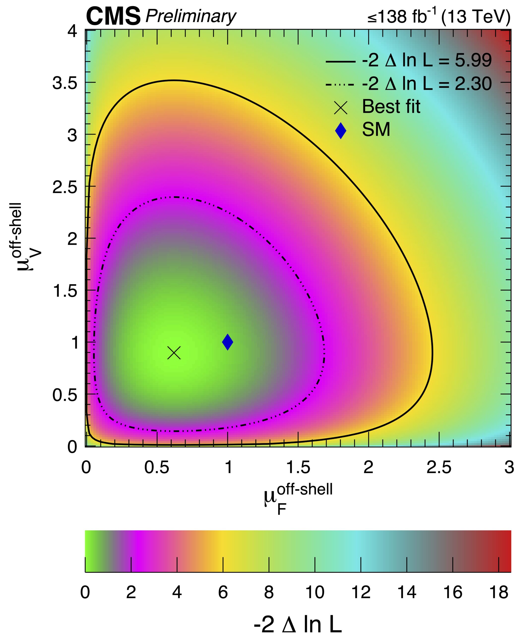
After a heavy load of sophisticated statistical analysis, the authors found that off-shell Higgs production happened at a rate consistent with SM predictions (Fig. 3). Using these off-shell events, they measured the Higgs width to be 3.2 (+2.4, -1.7) MeV, again consistent with the expectation of 4.1 MeV and a marked improvement upon the previously measured limit of 9.2 MeV.
Fig. 3: The best-fit “signal strength” parameters for off-shell Higgs production in two different modes: gluon fusion (x-axis, shown also in the leftmost Feynman diagram above) and associated production with a vector boson (y-axis). Signal strength measures how often a process occurs relative to the SM expectation, and a value of 1 means that it occurs at the rate predicted by the SM. In this case, the SM prediction (X) is within one standard deviation of the best fit signal strength (diamond).
Unfortunately, this result doesn’t hint at any new physics in the Higgs sector. It does, however, mark a significant step forward into the era of precision Higgs physics at ATLAS and CMS. With a mountain of data at our fingertips — and much more data to come in the next decade — we’ll soon find out what else the Higgs has to teach us.
In lieu of a typical HEP paper summary this month, I’m linking a comprehensive overview of the new results shown at this year’s Moriond conference, originally published in the CERN EP Department Newsletter. Since this includes the latest and greatest from all four experiments on the LHC ring (ATLAS, CMS, ALICE, and LHCb), you can take it as a sort of “state-of-the-field”. Here is a sneak preview:
“Every March, particle physicists around the world take two weeks to promote results, share opinions and do a bit of skiing in between. This is the Moriond tradition and the 52nd iteration of the conference took place this year in La Thuile, Italy. Each of the four main experiments on the LHC ring presented a variety of new and exciting results, providing an overview of the current state of the field, while shaping the discussion for future efforts.”
Read more in my article for the CERN EP Department Newsletter here!
The integrated luminosity of the LHC with proton-proton collisions in 2016 compared to previous years. Luminosity is a measure of a collider’s performance and is proportional to the number of collisions. The integrated luminosity achieved by the LHC in 2016 far surpassed expectations and is double that achieved at a lower energy in 2012.
It has been nearly five years since scientists at the LHC first observed a new particle that looked a whole lot like the highly sought after Higgs boson. In those five years, they have poked and prodded at every possible feature of that particle, trying to determine its identity once and for all. The conclusions? If this thing is an imposter, it’s doing an incredible job.
This new particle of ours really does seem to be the classic Standard Model Higgs. It is a neutral scalar, with a mass of about 125 GeV. All of its couplings with other SM particles are lying within uncertainty of their expected values, which is very important. You’ve maybe heard people say that the Higgs gives particles mass. This qualitative statement translates into an expectation that the Higgs coupling to a given particle is proportional to that particle’s mass. So probing the values of these couplings is a crucial task.
Figure 1: Best-fit results for the production signal strengths for the combination of ATLAS and CMS. Also shown for completeness are the results for each experiment. The error bars indicate the 1σ intervals.
Figure 1 shows the combined experimental measurements between ATLAS and CMS of Higgs decay signal strengths as a ratio of measurement to SM expectation. Values close to 1 means that experiment is matching theory. Looking at this plot, you might notice that a few of these values have significant deviations from 1, where our perfect Standard Model world is living. Specifically, the ttH signal strength is running a bit high. ttH is the production of a top pair and a Higgs from a single proton collision. There are many ways to do this, starting from the primary Higgs production mechanism of gluon-gluon fusion. Figure 2 shows some example diagrams that can produce this interesting ttH signature. While the deviations are a sign to physicists that maybe we don’t understand the whole picture.
Figure 2: Parton level Feynman diagrams of ttH at leading order.
Putting this in context with everything else we know about the Higgs, that top coupling is actually a key player in the Standard Model game. There is a popular unsolved mystery in the SM called the hierarchy problem. The way we understand the top quark contribution to the Higgs mass, we shouldn’t be able to get such a light Higgs, or a stable vacuum. Additionally, electroweak baryogenesis reveals that there are things about the top quark that we don’t know about.
Now that we know we want to study top-Higgs couplings, we need a way to characterize them. In the Standard Model, the coupling is purely scalar. However, in beyond the SM models, there can also be a pseudoscalar component, which violates charge-parity (CP) symmetry. Figure 3 shows a generic form for the term, where Cst is the scalar and Cpt is the pseudoscalar contribution. What we don’t know right away are the relative magnitudes of these two components. In the Standard Model, Cst = 1 and Cpt = 0. But theory suggests that there may be some non-zero value for Cpt, and that’s what we want to figure out.
Figure 3
Using simulations along with the datasets from Run 1 and Run 2 of the LHC, the authors of this paper investigated the possible values of Cst and Cpt. Figure 4 shows the updated bound. You can see from the yellow 2σ contour that the new limits on the values are |Cpt| < 0.37 and 0.85 < Cst < 1.20, extending the exclusions from Run 1 data alone. Additionally, the authors claim that the cross section of ttH can be enhanced up to 1.41 times the SM prediction. This enhancement could either come from a scenario where Cpt = 0 and Cst > 1, or the existence of a non-zero Cpt component.
Figure 4: The signal strength µtth at 13 TeV LHC on the plane of Cst and Cpt. The yellow contour corresponds to a 2σ limit.
Further probing of these couplings could come from the HL-LHC, through further studies like this one. However, examining the tH coupling in a future lepton collider would also provide valuable insights. The process e+e- à hZ contains a top quark loop. Thus one could make a precision measurement of this rate, simultaneously providing a handle on the tH coupling.
References and Further Reading:
“Enhanced Higgs associated production with a top quark pair in the NMSSM with light singlets”. arXiv hep-ph 02353
“Measurements of the Higgs boson production and decay rates and constraints on its couplings from a combined ATLAS and CMS analysis of the LHC pp collision data at √s = 7 and 8 TeV.” ATLAS-CONF-2015-044
After recovering from a dead-diphoton-excess induced depression (see here, here, and here for summaries) I am back to tell you a little more about something that actually does exist, our old friend Monsieur Higgs boson. All of the fuss over the past few months over a potential new particle at 750 GeV has perhaps made us forget just how special and interesting the Higgs boson really is, but as more data is collected at the LHC, we will surely be reminded of this fact once again (see Fig.1).
Figure 1: Monsieur Higgs boson struggles to understand the Higgs mechanism.
Previously I discussed how one of the best and most precise ways to study the Higgs boson is just by `shining light on it’, or more specifically via its decays to pairs of photons. Today I want to expand on another fantastic and precise way to study the Higgs which I briefly mentioned previously; Higgs decays to four charged leptons (specifically electrons and muons) shown in Fig.2. This is a channel near and dear to my heart and has a long history because it was realized, way before the Higgs was actually discovered at 125 GeV, to be among the best ways to find a Higgs boson over a large range of potential masses above around 100 GeV. This led to it being dubbed the “gold plated” Higgs discovery mode, or “golden channel”, and in fact was one of the first channels (along with the diphoton channel) in which the 125 GeV Higgs boson was discovered at the LHC.
Figure 2: Higgs decays to four leptons are mediated by the various physics effects which can enter in the grey blob. Could new physics be hiding in there?
One of the characteristics that makes the golden channel so valuable as a probe of the Higgs is that it is very precisely measured by the ATLAS and CMS experiments and has a very good signal to background ratio. Furthermore, it is very well understood theoretically since most of the dominant contributions can be calculated explicitly for both the signal and background. The final feature of the golden channel that makes it valuable, and the one that I will focus on today, is that it contains a wealth of information in each event due to the large number of observables associated with the four final state leptons.
Since there are four charged leptons which are measured and each has an associated four momentum, there are in principle 16 separate numbers which can be measured in each event. However, the masses of the charged leptons are tiny in comparison to the Higgs mass so we can consider them as massless (see Footnote 1) to a very good approximation. This then reduces (using energy-momentum conservation) the number of observables to 12 which, in the lab frame, are given by the transverse momentum, rapidity, and azimuthal angle of each lepton. Now, Lorentz invariance tells us that physics doesnt care which frame of reference we pick to analyze the four lepton system. This allows us to perform a Lorentz transformation from the lab frame where the leptons are measured, but where the underlying physics can be obscured, to the much more convenient and intuitive center of mass frame of the four lepton system. Due to energy-momentum conservation, this is also the center of mass frame of the Higgs boson. In this frame the Higgs boson is at rest and the $latex \emph{pairs}$ of leptons come out back to back (see Footnote 2) .
In this frame the 12 observables can be divided into 4 production and 8 decay (see Footnote 3). The 4 production variables are characterized by the transverse momentum (which has two components), the rapidity, and the azimuthal angle of the four lepton system. The differential spectra for these four variables (especially the transverse momentum and rapidity) depend very much on how the Higgs is produced and are also affected by parton distribution functions at hadron colliders like the LHC. Thus the differential spectra for these variables can not in general be computed explicitly for Higgs production at the LHC.
The 8 decay observables are characterized by the center of mass energy of the four lepton system, which in this case is equal to the Higgs mass, as well as two invariant masses associated with each pair of leptons (how one picks the pairs is arbitrary). There are also five angles ($latex \Theta, \theta_1, \theta_2$, Φ, Φ1) shown in Fig. 3 for a particular choice of lepton pairings. The angle $latex \Theta$ is defined as the angle between the beam axis (labeled by p or z) and the axis defined to be in the direction of the momentum of one of the lepton pair systems (labeled by Z1 or z’). This angle also defines the ‘production plane’. The angles $latex \theta_1, \theta_2$ are the polar angles defined in the lepton pair rest frames. The angle Φ1 is the azimuthal angle between the production plane and the plane formed from the four vectors of one of the lepton pairs (in this case the muon pair). Finally Φ is defined as the azimuthal angle between the decay planes formed out of the two lepton pairs.
Figure 3: Angular center of mass observables in Higgs to four lepton decays.
To a good approximation these decay observables are independent of how the Higgs boson is produced. Furthermore, unlike the production variables, the fully differential spectra for the decay observables can be computed explicitly and even analytically. Each of them contains information about the properties of the Higgs boson as do the correlations between them. We see an example of this in Fig. 4 where we show the one dimensional (1D) spectrum for the Φ variable under various assumptions about the CP properties of the Higgs boson.
Figure 4: Here I show various examples for the Φ differential spectrum assuming different possibilities for the CP properties of the Higgs boson.
This variable has long been known to be sensitive to the CP properties of the Higgs boson. An effect like CP violation would show up as an asymmetry in this Φ distribution which we can see in curve number 5 shown in orange. Keep in mind though that although I show a 1D spectrum for Φ, the Higgs to four lepton decay is a multidimensional differential spectrum of the 8 decay observables and all of their correlations. Thus though we can already see from a 1D projection for Φ how information about the Higgs is contained in these distributions, MUCH more information is contained in the fully differential decay width of Higgs to four lepton decays. This makes the golden channel a powerful probe of the detailed properties of the Higgs boson.
OK nibblers, hopefully I have given you a flavor of the golden channel and why it is valuable as a probe of the Higgs boson. In a future post I will discuss in more detail the various types of physics effects which can enter in the grey blob in Fig. 2. Until then, keep nibbling and don’t let dead diphotons get you down!
Footnote 1: If you are feeling uneasy about the fact that the Higgs can only “talk to” particles with mass and yet can decay to four massless (atleast approximately) leptons, keep in mind they do not interact directly. The Higgs decay to four charged leptons is mediated by intermediate particles which DO talk to the Higgs and charged leptons.
Footnote 2: More precisely, in the Higgs rest frame, the four vector formed out of the sum of the two four vectors of any pair of leptons which are chosen will be back to back with the four vector formed out of the sum of the second pair of leptons.
Footnote 3: This dividing into production and decay variables after transforming to the four lepton system center of mass frame (i.e. Higgs rest frame) is only possible in practice because all four leptons are visible and their four momentum can be reconstructed with very good precision at the LHC. This then allows for the rest frame of the Higgs boson to be reconstructed on an event by event basis. For final states with missing energy or jets which can not be reconstructed with high precision, transforming to the Higgs rest frame is in general not possible.
Today I want to discuss a slightly more advanced topic which I will not be able to explain in much detail, but goes by the name of the gauge Hierarchy problem or just the `the Hierarchy Problem‘. My main motivation is to simply make you curious enough that you will feel inspired to investigate it further for yourself since it is one of the outstanding problems in particle physics and one of the main motivations for the construction of the LHC. A second motivation is to bring to your attention a recent and exciting paper which proposes a potentially new solution to the hierarchy problem.
The hierarchy problem can roughly be stated as the problem of why the vacuum expectation value (VEV) of the Higgs boson, which determines the masses of the electroweak W and Z bosons, is so small compared to the highest energy scales thought to exist in the Universe. More specifically, the masses of the W and Z bosons (which define the weak scale) are roughly $latex \sim 10^{2}$ GeV (see Figure 1) in particle physics units (remember in these units mass = energy!).
The W boson as it finds to its astonishment that it has a mass of only about 100 GeV instead of $latex 10^{19}$ GeV as expected.
On the other hand the highest energy scale thought to exist in the Universe is the planck scale at $latex \sim 10^{19}$ GeV which is associated with the physics of gravity. Quantum field theory tells us that the Higgs VEV should get contributions from all energy scales (see Figure 2) so the question is why is the Higgs VEV, and thus the W and Z boson masses, a factor of roughly $latex \sim 10^{17}$ smaller than it should be?
The Higgs vacuum expectation value receives contributions from all energy scales.
In the Standard Model (SM) there is no solution to this problem. Instead one must rely on a spectacularly miraculous numerical cancellation among the parameters of the SM Lagrangian. Miraculous numerical `coincidences’ like this make us physicists feel uncomfortable to the point that we give it the special name of `fine tuning’. The hierarchy problem is thus also known as the fine tuning problem.
A search for a solution to this problem has been at the forefront of particle physics for close to 40 years. It is the aversion to fine tuning which leads most physicist to believe there must be new physics beyond the SM whose dynamics are responsible for keeping the Higgs VEV small. Proposals include supersymmetry, composite Higgs models, extra dimensions, as well as invoking the anthropic principle in the context of a multiverse. In many cases, these solutions require a variety of new particles at energies close to the weak scale ($latex \sim 100-1000$ GeV) and thus should be observable at the LHC. However the lack of evidence at the LHC for any physics beyond the SM is already bringing tension to many of these solutions. A solution which does not require new particles at the weak scale would thus be very attractive.
Recently a novel mechanism, which goes by the name of $latex \emph{cosmological relaxation of the electroweak scale}$, has been proposed which potentially offers such a solution. The details (which physicists are currently still digesting) are well beyond the scope of this blog. I will just mention that the mechanism incorporates two previously proposed mechanisms known as inflation$latex ^1$ and the QCD axion$latex ^2$ which solve other known problems. These are combined with the SM in a novel way such that the weak scale can arise naturally in our universe without any fine tuning and without new particles at the weak scale (or multiple universes)! And as a bonus, the axion in this mechanism (referred to as the `relaxion’) makes a good dark matter candidate!
Whether or not this mechanism turns out to be a solution to the hierarchy problem will of course require experimental tests and further theoretical scrutiny, but its a fascinating idea which combines aspects of quantum field theory and general relativity so I hope it will serve as motivation for you to begin learning more about these subjects!
$latex \bf{Footnotes:}$
1. Inflation is a theorized period of exponential accelerated expansion of our Universe in the moments just after the big bang. It was proposed as a solution to the problems of why our Universe is so flat and (mostly) homogenous while also explaining the structure we see throughout the Universe and in the cosmic microwave background.
2. Axions are particles proposed to explain why the amount of CP violation in the QCD sector in the SM is so small, which is known as the `strong CP problem‘.