
This is the second part of our coverage of the P5 report and its implications for particle physics. To read the first part, click here
One of the thorniest questions in particle physics is ‘What comes after the LHC?’. This was one of the areas people were most uncertain what the P5 report would say. Globally, the field is trying to decide what to do once the LHC winds down in ~2040 While the LHC is scheduled to get an upgrade in the latter half of the decade and run until the end of the 2030’s, the field must start planning now for what comes next. For better or worse, big smash-y things seem to capture a lot of public interest, so the debate over what large collider project to build has gotten heated. Even Elon Musk is tweeting (X-ing?) memes about it.
Famously, the US’s last large accelerator project, the Superconducting Super Collider (SSC), was cancelled in the ’90s partway through its construction. The LHC’s construction itself often faced perilous funding situations, and required a CERN to make the unprecedented move of taking a loan to pay for its construction. So no one takes for granted that future large collider projects will ultimately come to fruition.
Desert or Discovery?
When debating what comes next, dashed hopes of LHC discoveries are top of mind. The LHC experiments were primarily designed to search for the Higgs boson, which they successfully found in 2012. However, many had predicted (perhaps over-confidently) it would also discover a slew of other particles, like those from supersymmetry or those heralding extra-dimensions of spacetime. These predictions stemmed from a favored principle of nature called ‘naturalness’ which argued additional particles nearby in energy to the Higgs were needed to keep its mass at a reasonable value. While there is still much LHC data to analyze, many searches for these particles have been performed so far and no signs of these particles have been seen.
These null results led to some soul-searching within particle physics. The motivations behind the ‘naturalness’ principle that said the Higgs had to be accompanied by other particles has been questioned within the field, and in New York Times op-eds.
No one questions that deep mysteries like the origins of dark matter, matter anti-matter asymmetry, and neutrino masses, remain. But with the Higgs filling in the last piece of the Standard Model, some worry that answers to these questions in the form of new particles may only exist at energy scales entirely out of the reach of human technology. If true, future colliders would have no hope of

The situation being faced now is qualitatively different than the pre-LHC era. Prior to the LHC turning on, ‘no lose theorems’, based on the mathematical consistency of the Standard Model, meant that it had to discover the Higgs or some other new particle like it. This made the justification for its construction as bullet-proof as one can get in science; a guaranteed Nobel prize discovery. But now with the last piece of the Standard Model filled in, there are no more free wins; guarantees of the Standard Model’s breakdown don’t occur until energy scales we would need solar-system sized colliders to probe. Now, like all other fields of science, we cannot predict what discoveries we may find with future collider experiments.
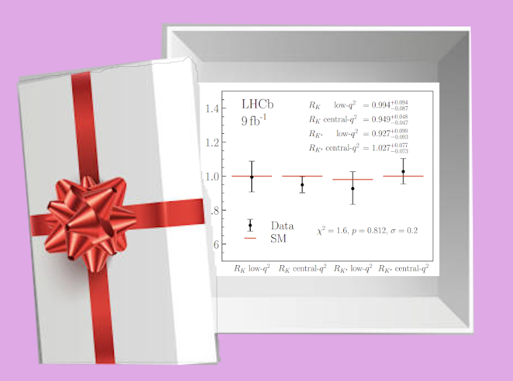
Still, optimists hope, and have their reasons to believe, that nature may not be so unkind as to hide its secrets behind walls so far outside our ability to climb. There are compelling models of dark matter that live just outside the energy reach of the LHC, and predict rates too low for direct detection experiments, but would be definitely discovered or ruled out by high energy colliders. The nature of the ‘phase transition’ that occurred in the very early universe, which may explain the prevalence of matter over anti-matter, can also be answered. There are also a slew of experimental ‘hints‘, all of which have significant question marks, but could point to new particles within the reach of a future collider.
Many also just advocate for building a future machine to study nature itself, with less emphasis on discovering new particles. They argue that even if we only further confirm the Standard Model, it is a worthwhile endeavor. Though we calculate Standard Model predictions for high energies, unless they are tested in a future collider we will not ‘know’ how if nature actually works like this until we test it in those regimes. They argue this is a fundamental part of the scientific process, and should not be abandoned so easily. Chief among the untested predictions are those surrounding the Higgs boson. The Higgs is a central somewhat mysterious piece of the Standard Model but is difficult to measure precisely in the noisy environment of the LHC. Future colliders would allow us to study it with much better precision, and verify whether it behaves as the Standard Model predicts or not.
Projects
These theoretical debates directly inform what colliders are being proposed and what their scientific case is.
Many are advocating for a “Higgs factory”, a collider of based on clean electron-positron collisions that could be used to study the Higgs in much more detail than the messy proton collisions of the LHC. Such a machine would be sensitive to subtle deviations of Higgs behavior from Standard Model predictions. Such deviations could come from the quantum effects of heavy, yet-undiscovered particles interacting with the Higgs. However, to determine what particles are causing those deviations, its likely one would need a new ‘discovery’ machine which has high enough energy to produce them.
Among the Higgs factory options are the International Linear Collider, a proposed 20km linear machine which would be hosted in Japan. ILC designs have been ‘ready to go’ for the last 10 years but the Japanese government has repeated waffled on whether to approve the project. Sitting in limbo for this long has led to many being pessimistic about the projects future, but certainly many in the global community would be ecstatic to work on such a machine if it was approved.

Alternatively, some in the US have proposed building a linear collider based on a ‘cool copper’ cavities (C3) rather than the standard super conducting ones. These copper cavities can achieve more acceleration per meter than the standard super conducting ones, meaning a linear Higgs factory could be constructed with a reduced 8km footprint. A more compact design can significantly cut down on infrastructure costs that governments usually don’t like to use their science funding on. Advocates had proposed it as a cost-effective Higgs factory option, whose small footprint means it could potentially hosted in the US.
The Future-Circular-Collider (FCC), CERN’s successor to the LHC, would kill both birds with one extremely long stone. Similar to the progression from LEP to the LHC, this new proposed 90km collider would run as Higgs factory using electron-positron collisions starting in 2045 before eventually switching to a ~90 TeV proton-proton collider starting in ~2075.

Such a machine would undoubtably answer many of the important questions in particle physics, however many have concerns about the huge infrastructure costs needed to dig such a massive tunnel and the extremely long timescale before direct discoveries could be made. Most of the current field would not be around 50 years from now to see what such a machine finds. The Future-Circular-Collider (FCC), CERN’s successor to the LHC, would kill both birds with one extremely long stone. Similar to the progression from LEP to the LHC, this new proposed 90km collider would run as Higgs factory using electron-positron collisions starting in 2045 before eventually switching to a ~90 TeV proton-proton collider starting in ~2075. Such a machine would undoubtably answer many of the important questions in particle physics, however many have concerns about the extremely long timescale before direct discoveries could be made. Most of the current field would not be around 50 years from now to see what such a machine finds. The FCC is also facing competition as Chinese physicists have proposed a very similar design (CEPC) which could potentially start construction much earlier.
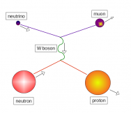
During the snowmass process many in the US starting pushing for an ambitious alternative. They advocated a new type of machine that collides muons, the heavier cousin of electrons. A muon collider could reach the high energies of a discovery machine while also maintaining a clean environment that Higgs measurements can be performed in. However, muons are unstable, and collecting enough of them into formation to form a beam before they decay is a difficult task which has not been done before. The group of dedicated enthusiasts designed t-shirts and Twitter memes to capture the excitement of the community. While everyone agrees such a machine would be amazing, the key technologies necessary for such a collider are less developed than those of electron-positron and proton colliders. However, if the necessary technological hurdles could be overcome, such a machine could turn on decades before the planned proton-proton run of the FCC. It can also presents a much more compact design, at only 10km circumfrence, roughly three times smaller than the LHC. Advocates are particularly excited that this would allow it to be built within the site of Fermilab, the US’s flagship particle physics lab, which would represent a return to collider prominence for the US.

Deliberation & Decision
This plethora of collider options, each coming with a very different vision of the field in 25 years time led to many contentious debates in the community. The extremely long timescales of these projects led to discussions of human lifespans, mortality and legacy being much more being much more prominent than usual scientific discourse.
Ultimately the P5 recommendation walked a fine line through these issues. Their most definitive decision was to recommend against a Higgs factor being hosted in the US, a significant blow to C3 advocates. The panel did recommend US support for any international Higgs factories which come to fruition, at a level ‘commensurate’ with US support for the LHC. What exactly ‘comensurate’ means in this context I’m sure will be debated in the coming years.
However, the big story to many was the panel’s endorsement of the muon collider’s vision. While recognizing the scientific hurdles that would need to be overcome, they called the possibility of muon collider hosted in the US a scientific ‘muon shot‘, that would reap huge gains. They therefore recommended funding for R&D towards they key technological hurdles that need to be addressed.
Because the situation is unclear on both the muon front and international Higgs factory plans, they recommended a follow up panel to convene later this decade when key aspects have clarified. While nothing was decided, many in the muon collider community took the report as a huge positive sign. While just a few years ago many dismissed talk of such a collider as fantastical, now a real path towards its construction has been laid down.

While the P5 report is only one step along the path to a future collider, it was an important one. Eyes will now turn towards reports from the different collider advocates. CERN’s FCC ‘feasibility study’, updates around the CEPC and, the International Muon Collider Collaboration detailed design report are all expected in the next few years. These reports will set up the showdown later this decade where concrete funding decisions will be made.
For those interested the full report as well as executive summaries of different areas can be found on the P5 website. Members of the US particle physics community are also encouraged to sign the petition endorsing the recommendations here.


