Month: September 2020

Article Title: Inclusive search for highly boosted Higgs bosons decaying to bottom quark-antiquark pairs in proton-proton collisions at √s= 13 TeV

Authors: The CMS Collaboration

Reference arxiv:2006.13251

Since the discovery of the Higgs boson one of the main tasks of the LHC experiments has been to study all of its properties and see if they match the Standard Model predictions. Most of this effort has gone into characterizing the different ways the Higgs can be produced (‘production modes’) and how often it decays into its different channels (‘branching ratios’). However if you are a fan of Sonic the Hedgehog, you might have also wondered ‘How often does the Higgs go really fast?’. While that might sound like a very silly question, it is actually a very interesting one to study, and what has been done in this recent CMS analysis.

But what does it mean for the Higgs to ‘go fast’? You might have thought that the Higgs moves quite slowly because it is the 2nd heaviest fundamental particle we know of, with a mass around 125 times that of a proton. But sometimes very energetic LHC collisions can have enough energy to not only to make a Higgs boson but give it a ‘kick’ as well. If the Higgs is produced with enough momentum that it moves away from the beamline at a speed relatively close to the speed of light we call it ‘boosted’.

Not only are these boosted Higgs just a very cool thing to study, they can also be crucial to seeing the effects of new particles interacting with the Higgs. If there was a new heavy particle interacting with the Higgs during its production you would expect to see the largest effect on the rates of Higgs production at high momentum. So if you don’t look specifically at the rates of these boosted Higgs production you might miss this clue of new physics.

Another benefit is that when the Higgs is produced with a boost it significantly changes its experimental signature, often making it easier to spot. The Higgs’s favorite decay channel, its decay into a pair of bottom quarks, is notoriously difficult to study. A bottom quark, like any quark produced in an LHC collision, does not reach the detector directly, but creates a huge shower of particles known as a jet. Because bottom quarks live long enough to travel a little bit away from the beam interaction point before decaying, their jets start a little bit displaced compared to other jets. This allows experimenters to ‘tag’ jets likely to have come from bottom quarks. In short, the experimental signature of this Higgs decay is two jets that look bottom-like. This signal is very hard to find amidst a background of jets produced via the strong force which occur at rates orders of magnitude more often than Higgs production. 

 

 But when a particle with high momentum decays, its decay products will be closer together in the reference frame of the detector. When the Higgs is produced with a boost, the two bottom quarks form a single large jet rather than two separated jets. This single jet should have the signature of two b quarks inside of it rather than just one. What’s more, the distribution of particles within the jet should form 2 distinct ‘prongs’, one coming from each of the bottom quarks, rather than a single core that would be characteristic of a jet produced by a single quark or gluon. These distinct characteristics help analyzers pick out events more likely to be boosted Higgs from regular QCD events. 

The end goal is to select events with these characteristics and then look for a excess of events that have an invariant mass of 125 GeV, which would be the tell-tale sign of the Higgs. When this search was performed they did see such a bump, an excess over the estimated background with a significance of 2.5 standard deviations. This is actually a stronger signal than they were expecting to see in the Standard Model. They measure the strength of the signal they see to be 3.7 ± 1.6 times the strength predicted by the Standard Model. 

The analyzers then study this excess more closely by checking the signal strength in different regions of Higgs momentum. What they see is that the excess is coming from the events with the highest momentum Higgs’s.  The significance of the excess of high momentum Higgs’s above the Standard Model prediction is about 2 standard deviations.

So what we should we make of these extra speedy Higgs’s? Well first of all, the deviation from the Standard Model it is not very statistically significant yet, so it may disappear with further study. ATLAS is likely working on a similar measurement with their current dataset so we will wait to see if they confirm this excess. Another possibility is that the current predictions for the Standard Model, which are based on difficult perturbative QCD calculations, may be slightly off. Theorists will probably continue make improvements to these predictions in the coming years. But if we continue to see the same effect in future measurements, and the Standard Model prediction doesn’t budge, these speedy Higgs’s may turn out to be our first hint of the physics beyond the Standard Model!

Further Reading:

“First Evidence the Higgs Talks to Other Generations“: previous ParticleBites post on recent Higgs boson news

“A decade of advances in jet substructure“: Cern Courier article on techniques to identify boosted particles (like the Higgs) decaying into jets

“Jets: From Energy Deposits to Physics Objects“: previous ParticleBites post on how jets are measured

Article title: Bayesian Neural Networks for Fast SUSY Predictions

Authors: B. S. Kronheim, M. P. Kuchera, H. B. Prosper, A. Karbo

Reference: https://arxiv.org/abs/2007.04506

It has been a while since we have graced these parts with the sounds of the attractive yet elusive superhero named SUSY. With such an arduous history of experimental effort, supersymmetry still remains unseen by the eyes of even the most powerful colliders. Though in the meantime, phenomenologists and theorists continue to navigate the vast landscape of model parameters with hopes of narrowing in on the most intriguing predictions – even connecting dark matter into the whole mess.

How vast you may ask? Well the ‘vanilla’ scenario, known as the Minimal Supersymmetric Standard Model (MSSM) – containing partner particles for each of those of the Standard Model – is chock-full of over 100 free parameters. This makes rigorous explorations of the parameter space not only challenging to interpret, but also computationally expensive. In fact, the standard practice is to confine oneself to a subset of the parameter space, using suitable justifications, and go ahead to predict useful experimental observables like collider production rates or particle masses. One of these popular motivations is known as the phenoneological MSSM (pMSSM), which reduces the huge parameter area to just less than 20 by assuming the absence of things like SUSY-driven CP-violation, flavour changing neutral currents (FCNCs) and differences between first and second generation SUSY particles. With this in the toolbox, computations become comparatively more feasible, with just enough complexity to make solid but interesting predictions.

But even coming from personal experience, these spaces can still be typically be rather tedious to work through – especially since many parameter selections are theoretically nonviable and/or in disagreement with previously well-established experimental observables, like the mass of the Higgs Boson. Maybe there is a faster way?

Machine learning has shared a successful history with a lot of high-energy physics applications, particularly those with complex dynamics like SUSY. One particularly useful application, at which machine learning is very accomplished at, is classification of points as excluded or not excluded based on searches at the LHC by ATLAS and CMS.

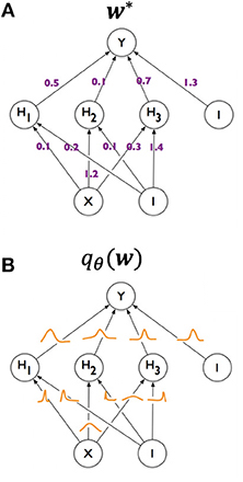
In the considered paper, a special type of Neural Network (NN) known as a Bayesian Neural Network (BNN) is used, which notably rely on probablistic certainty of classification rather than simply classifying a result as one thing or the other.

In a typical NN there is a space of adjustable parameters (often called “features”) and a list of “targets” for the model to learn classification from. In this particular case, the model parameters are of course the features to learn from – these mainly include mass parameters for the different superparticles in the spectrum. These are mapped to three different predictions or targets that can be computed from these parameters:

1. The mass of the lightest, neutral Higgs Boson (the 125 GeV one)
2. The cross sections of processes involving the superpartners to the elecroweak guage bosons (typically called the neutralinos and charginos – I will let you figure out which ones are the charged and neutral ones)
3. Whether the point is actually valid or not (or maybe theoretically consistent is a better way to put it).

Of course there is an entire suite of programs designed to carry out these calculations, which are usually done point by point in the parameter space of the pMSSM, and hence these would be used to construct the training data sets for the algorithm to learn from – one data set for each of the predictions listed above.

But how do we know our model is trained properly once we have finished the learning process? There are a number of metrics that are very commonly used to determine whether a machine learning algorithm can correctly classify the results of a set of parameter points. The following table sums up the four different types of classifications that could be made on a set of data.

The typical measures employed using this table are the precision, recall and F1 score which are in practice readily defined as:

In predicting the validity of points, the recall especially will tell us the fraction of valid points that will be correctly identified by the algorithm. For example, the metrics for this validity data set are shown in Table 2.

With a higher Recall but lower precision for the 3 standard deviation cutoff it is clear that points with a larger uncertainty will be classified as valid in this case. Such a scenario would be useful in calculating further properties like the mass spectrum, but not neccesarily as the best classifier.

Similarly with the data set used to compute cross sections, the standard deviation can be used for points where the predictions are quite uncertain. On average their calculations revealed just over 3% percent error with the actual value of the cross section. Not to be outdone, in calculating the Higgs boson mass, within 2 GeV deviation of 125 GeV, the precision of the BNN was found to be 0.926 with a recall of 0.997, showing that very few parameter points that are actually conistent with the light neutral Higgs will actually be removed.

In the end, our whole purpose was to provide reliable SUSY predictions at a fraction of the time. It is well known that NNs provide relatively fast calculation, especially when utilizing powerful hardware, and in this case could acheive up to over 16 million times faster in computing a single point than standard SUSY software! Finally, it is worth to note that neural networks are highly scalable and so predictions from the 19-dimensional pMSSM are but one of the possibilities for NNs in calculating SUSY observables.

Futher Reading

[1] Bayesian Neural Networks and how they differ from traditional NNs: https://towardsdatascience.com/making-your-neural-network-say-i-dont-know-bayesian-nns-using-pyro-and-pytorch-b1c24e6ab8cd

[2] More on machine learning and A.I. and its application to SUSY: https://arxiv.org/abs/1605.02797