A Massive W for CDF

This is part two of our coverage of the CDF W mass measurement, discussing how the measurement was done. Read about the implications of this result in our sister post here

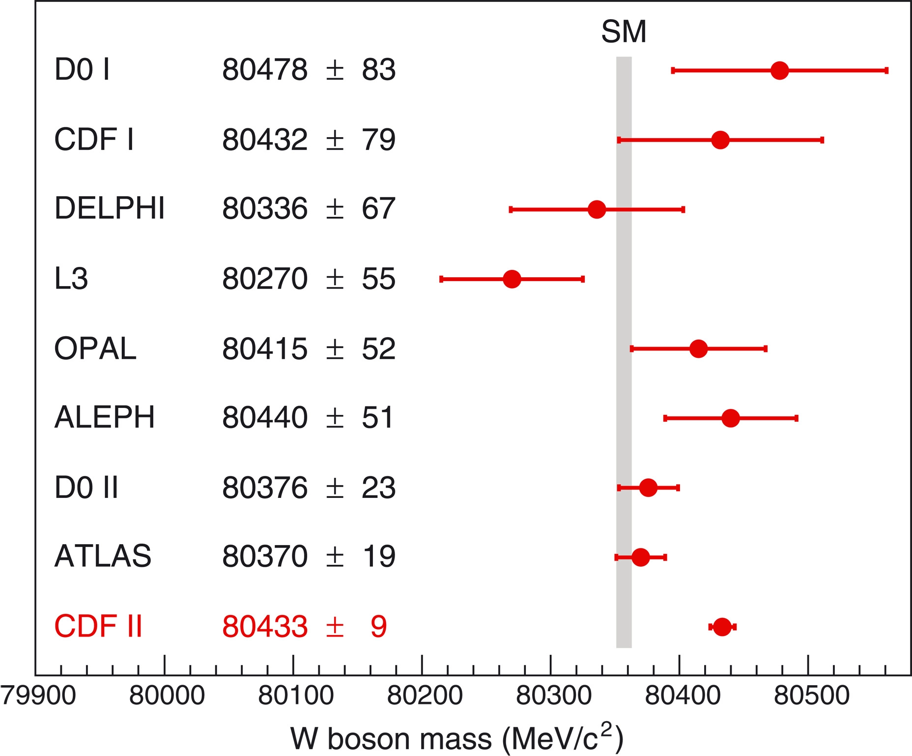
Last week, the CDF collaboration announced the most precise measurement of the W boson’s mass to date. After nearly ten years of careful analysis, the W weighed in at 80,433.5 ± 9.4 MeV: a whopping seven standard deviations away from the Standard Model expectation! This result quickly became the talk of the town among particle physicists, and there are already dozens of arXiv papers speculating about what it means for the Standard Model. One of the most impressive and hotly debated aspects of this measurement is its high precision, which came from an extremely careful characterization of the CDF detector and recent theoretical developments in modeling proton structure. In this post, I’ll describe how they made the measurement and the clever techniques they used to push down the uncertainties.

The new CDF measurement of the W boson mass. The center of the red ellipse corresponds to the central values of the measured W mass (y-coordinate) and top quark mass (x-coordinate, from other experiments). The purple line shows the Standard Model constraint on the W mass as a function of the top mass, and the border of the red ellipse is the one standard deviation boundary around the measurement.

The imaginatively titled “Collider Detector at Fermilab” (CDF) collected proton-antiproton collision data at Fermilab’s Tevatron accelerator for over 20 years, until the Tevatron shut down in 2011. Much like ATLAS and CMS, CDF is made of cylindrical detector layers, with the innermost charged particle tracker and adjacent electromagnetic calorimeter (ECAL) being most important for the W mass measurement. The Tevatron ran at a center of mass energy of 1.96 TeV — much lower than the LHC’s 13 TeV — which enabled a large reduction in the “theoretical uncertainties” on the measurement. Physicists use models called “parton distribution functions” (PDFs) to calculate how a proton’s momentum is distributed among its constituent quarks, and modern PDFs make very good predictions at the Tevatron’s energy scale. Additionally, W boson production in proton-antiproton collisions doesn’t involve any gluons, which are a major source of uncertainty in PDFs (LHC collisions are full of gluons, making for larger theory uncertainty in LHC W mass measurements).

A cutaway view of the CDF detector. The innermost tracking detector (yellow) reconstructs the trajectories of charged particles, and the nearby electromagnetic calorimeter (red) collects energy deposits from photons and charged particles (e.g. electrons). The tracker and EM Cal were both central in the W mass measurement.

Armed with their fancy PDFs, physicists set out to measure the W mass in the same way as always: by looking at its decay products! They focused on the leptonic channel, where the W decays to a lepton (electron or muon) and its associated neutrino. This clean final state is easy to identify in the detector and allows for a high-purity, low-background signal selection. The only sticking point is the neutrino, which flies out of the detector completely undetected. Thankfully, momentum conservation allowed them to reconstruct the neutrino’s transverse momentum (pT) from the rest of the visible particles produced in the collision. Combining this with the lepton’s measured momentum, they reconstructed the “transverse mass” of the W — an important observable for estimating its true mass.

A leptonic decay of the W boson, where it decays to an electron and an electron antineutrino. This channel, along with the muon + muon antineutrino channel, formed the basis of CDF’s W mass measurement.

Many of the key observables for this measurement flow from the lepton’s momentum, which means it needs to be measured very carefully! The analysis team calibrated their energy and momentum measurements by using the decays of other Standard Model particles: the ϒ(1S) and J/ψ mesons, and the Z boson. These particles’ masses are very precisely known from other experiments, and constraints from these measurements helped physicists understand how accurately CDF reconstructs a particle’s energy. For momentum measurements in the tracker, they reconstructed the ϒ(1S) and J/ψ masses from their decays to muon-antimuon pairs inside CDF, and compared CDF-measured masses to their known values from other experiments. This allowed them to calculate a correction factor to apply to track momenta. For ECAL energy measurements, they looked at samples of Z and W bosons decaying to electrons, and measured ratio of energy deposited in the ECAL (E) to the momentum measured in the tracker (p). The shape of the E/p distribution then allowed them to calculate an energy calibration for the ECAL.

Left: the fractional deviation of the measured muon momentum relative to its true momentum (y-axis), as a function of the muon’s average inverse transverse momentum. Data from ϒ(1S), J/ψ, and Z decays are shown, and the fit line (in black) has a slope consistent with zero. This indicates that there is no significant mismodeling of the energy lost by a particle flying through the detector. Right: the distribution of the ratio energy measured in the ECAL to momentum measured in the tracker. The shape of the peak and tail are used to calibrate the ECAL energy measurements.

To make sure their tracker and ECAL calibrations worked correctly, they applied them in measurements of the Z boson mass in the electron and muon decay channels. Thankfully, their measurements were consistent with the world average in both channels, providing an important cross-check of their calibration strategy.

Having done everything humanly possible to minimize uncertainties and calibrate their measurements, the analysis team was finally ready to measure the W mass. To do this, they simulated W boson events with many different settings for the W mass (an additional mountain of effort went into ensuring that the simulations were as accurate as possible!). At each mass setting, they extracted “template” distributions of the lepton pT, neutrino pT, and W boson transverse mass, and fit each template to the distribution measured in real CDF data. The templates that best fit the measured data correspond to CDF’s measured value of the W mass (plus some additional legwork to calculate uncertainties)

The reconstructed W boson transverse mass distribution in the muon + muon antineutrino decay channel. The best-fit template (red) is plotted along with the background distribution (gray) and the measured data (black points).

After years of careful analysis, CDF’s measurement of mW = 80,433.5 ± 9.4 MeV sticks out like a sore thumb. If it stands up to the close scrutiny of the particle physics community, it’s further evidence that something new and mysterious lies beyond the Standard Model. The only way to know for sure is to make additional measurements, but in the meantime we’ll all be happily puzzling over what this might mean.

CDF’s W mass measurement (bottom), shown alongside results from other experiments and the SM expectation (gray).

Read More

Quanta Magazine’s coverage of the measurement

A recorded talk from the Fermilab Wine & Cheese seminar covering the result in great detail

The Higgs Comes Out of its Shell

Title : “First evidence for off-shell production of the Higgs boson and measurement of its width”

Authors : The CMS Collaboration

Link : https://arxiv.org/abs/2202.06923

CMS Analysis Summary : https://cds.cern.ch/record/2784590?ln=en

If you’ve met a particle physicist in the past decade, they’ve almost certainly told you about the Higgs boson. Since its discovery in 2012, physicists have been busy measuring as many of its properties as the ATLAS and CMS datasets will allow, including its couplings to other particles (e.g. bottom quarks or muons) and how it gets produced at the LHC. Any deviations from the standard model (SM) predictions might signal new physics, so people are understandably very eager to learn as much as possible about the Higgs.

Amidst all the talk of Yukawa couplings and decay modes, it might occur to you to ask a seemingly simpler question: what is the Higgs boson’s lifetime? This turns out to be very difficult to measure, and it was only recently — nearly 10 years after the Higgs discovery — that the CMS experiment released the first measurement of its lifetime.

The difficulty lies in the Higgs’ extremely short lifetime, predicted by the standard model to be around 10⁻²² seconds. This is far shorter than anything we could hope to measure directly, so physicists instead measured a related quantity: its width. According to the Heiseinberg uncertainty principle, short-lived particles can have significant uncertainty in their energy. This means that whenever we produce a Higgs boson at the LHC and reconstruct its mass from its decay products, we’ll measure a slightly different mass each time. If you make a histogram of these measurements, its shape looks like a Breit-Wigner distribution (Fig. 1) peaked at the nominal mass and with a characteristic width .

Fig. 1: A Breit-Wigner curve, which describes the distribution of masses that a particle takes on when it’s produced at the LHC. The peak sits at the particle’s nominal mass, and production within the width is most common (“on-shell”). The long tails allow for rare production far from the peak (“off-shell”).

So, the measurement should be easy, right? Just measure a bunch of Higgs decays, make a histogram of the mass, and run a fit! Unfortunately, things don’t work out this way. A particle’s width and lifetime are inversely proportional, meaning an extremely short-lived particle will have a large width and vice-versa. For particles like the Z boson — which lives for about 10⁻²⁵ seconds — we can simply extract its width from its mass spectrum. The Higgs, however, sits in a sweet spot of experimental evasion: its lifetime is too short to measure, and the corresponding width (about 4 MeV) cannot be resolved by our detectors, whose resolution is limited to roughly 1 GeV.

To overcome this difficulty, physicists relied on another quantum mechanical quirk: “off-shell” Higgs production. Most of the time, a Higgs is produced on-shell, meaning its reconstructed mass will be close to the Breit-Wigner peak. In rare cases, however, it can be produced with a mass very far away from its nominal mass (off-shell) and undergo decays that are otherwise energetically forbidden. Off-shell production is incredibly rare, but if you can manage to measure the ratio of off-shell to on-shell production rates, you can deduce the Higgs width!

Have we just replaced one problem (a too-short lifetime) with another one (rare off-shell production)? Thankfully, the Breit-Wigner distribution saves the day once again. The CMS analysis focused on a Higgs decaying to a pair of Z bosons (Fig. 2, left), one of which must be produced off-shell (the Higgs mass is 125 GeV, whereas each Z is 91 GeV). The Z bosons have a Breit-Wigner peak of their own, however, which enhances the production rate of very off-shell Higgs bosons that can decay to a pair of on-shell Zs. The enhancement means that roughly 10% of H → ZZ decays are expected to involve an off-shell Higgs, which is a large enough fraction to measure with the present-day CMS dataset!

Fig. 2: The signal process involving a Higgs decay to Z bosons (left), and background ZZ production without the Higgs (right)

To measure the off-shell H → ZZ rate, physicists looked at events where one Z boson decays to a pair of leptons and the other to a pair of neutrinos. The neutrinos escape the detector without depositing any energy, generating a large missing transverse momentum which helps identify candidate Higgs events. Using the missing momentum as a proxy for the neutrinos’ momentum, they reconstruct a “transverse mass” for the off-shell Higgs boson. By comparing the observed transverse mass spectrum to the expected “continuum background” (Z boson pairs produced via other mechanisms, e.g. Fig. 2, right) and signal rate, they are able to extract the off-shell production rate.

After a heavy load of sophisticated statistical analysis, the authors found that off-shell Higgs production happened at a rate consistent with SM predictions (Fig. 3). Using these off-shell events, they measured the Higgs width to be 3.2 (+2.4, -1.7) MeV, again consistent with the expectation of 4.1 MeV and a marked improvement upon the previously measured limit of 9.2 MeV.

Fig. 3: The best-fit “signal strength” parameters for off-shell Higgs production in two different modes: gluon fusion (x-axis, shown also in the leftmost Feynman diagram above) and associated production with a vector boson (y-axis). Signal strength measures how often a process occurs relative to the SM expectation, and a value of 1 means that it occurs at the rate predicted by the SM. In this case, the SM prediction (X) is within one standard deviation of the best fit signal strength (diamond).

Unfortunately, this result doesn’t hint at any new physics in the Higgs sector. It does, however, mark a significant step forward into the era of precision Higgs physics at ATLAS and CMS. With a mountain of data at our fingertips — and much more data to come in the next decade — we’ll soon find out what else the Higgs has to teach us.

Read More

“Life of the Higgs Boson” – Coverage of this result from the CMS Collaboration

“Most Particles Decay — But Why?” – An interesting article by Matt Strassler explaining why (some) particles decay

“The Physics Still Hiding in the Higgs Boson” – A Quanta article on what we can learn about new physics by measuring Higgs properties