The Delirium over Beryllium

Article: Particle Physics Models for the 17 MeV Anomaly in Beryllium Nuclear Decays
Authors: J.L. Feng, B. Fornal, I. Galon, S. Gardner, J. Smolinsky, T. M. P. Tait, F. Tanedo
Reference: arXiv:1608.03591 (Submitted to Phys. Rev. D)
See also this Latin American Webinar on Physics recorded talk.
Also featuring the results from:
— Gulyás et al., “A pair spectrometer for measuring multipolarities of energetic nuclear transitions” (description of detector; 1504.00489NIM)
— Krasznahorkay et al., “Observation of Anomalous Internal Pair Creation in 8Be: A Possible Indication of a Light, Neutral Boson”  (experimental result; 1504.01527PRL version; note PRL version differs from arXiv)
— Feng et al., “Protophobic Fifth-Force Interpretation of the Observed Anomaly in 8Be Nuclear Transitions” (phenomenology; 1604.07411; PRL)

Editor’s note: the author is a co-author of the paper being highlighted. 

Recently there’s some press (see links below) regarding early hints of a new particle observed in a nuclear physics experiment. In this bite, we’ll summarize the result that has raised the eyebrows of some physicists, and the hackles of others.

A crash course on nuclear physics

Nuclei are bound states of protons and neutrons. They can have excited states analogous to the excited states of at lowoms, which are bound states of nuclei and electrons. The particular nucleus of interest is beryllium-8, which has four neutrons and four protons, which you may know from the triple alpha process. There are three nuclear states to be aware of: the ground state, the 18.15 MeV excited state, and the 17.64 MeV excited state.

Beryllium-8 excited nuclear states. The 18.15 MeV state (red) exhibits an anomaly. Both the 18.15 MeV and 17.64 states decay to the ground through a magnetic, p-wave transition. Image adapted from Savage et al. (1987).

Most of the time the excited states fall apart into a lithium-7 nucleus and a proton. But sometimes, these excited states decay into the beryllium-8 ground state by emitting a photon (γ-ray). Even more rarely, these states can decay to the ground state by emitting an electron–positron pair from a virtual photon: this is called internal pair creation and it is these events that exhibit an anomaly.

The beryllium-8 anomaly

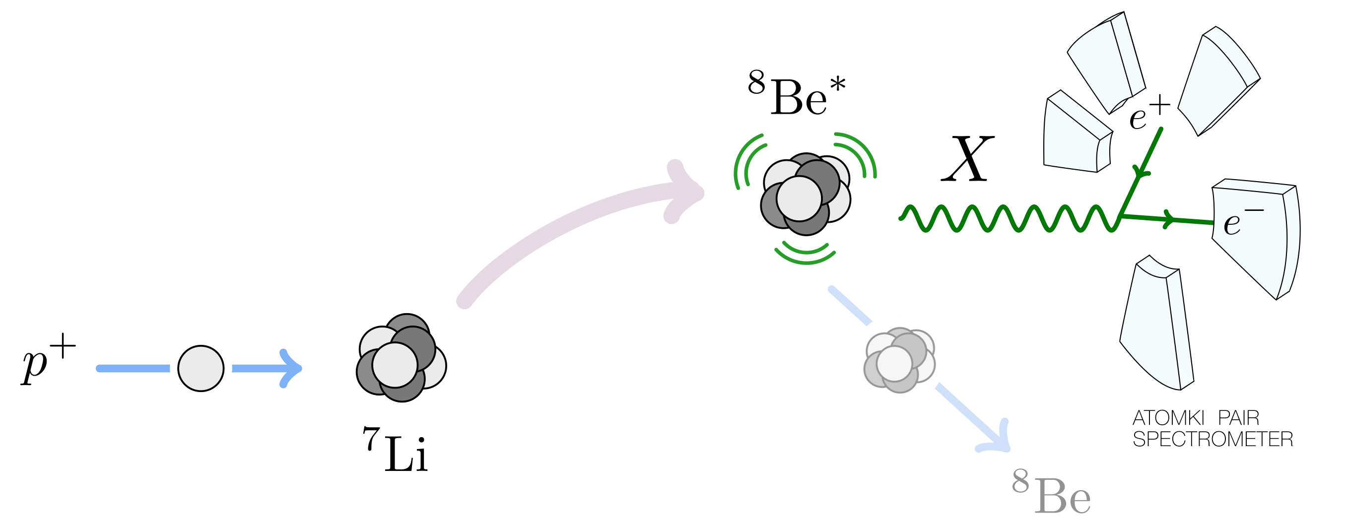
Physicists at the Atomki nuclear physics institute in Hungary were studying the nuclear decays of excited beryllium-8 nuclei. The team, led by Attila J. Krasznahorkay, produced beryllium excited states by bombarding a lithium-7 nucleus with protons.

Preparation of beryllium-8 excited state
Beryllium-8 excited states are prepare by bombarding lithium-7 with protons.

The proton beam is tuned to very specific energies so that one can ‘tickle’ specific beryllium excited states. When the protons have around 1.03 MeV of kinetic energy, they excite lithium into the 18.15 MeV beryllium state. This has two important features:

  1. Picking the proton energy allows one to only produce a specific excited state so one doesn’t have to worry about contamination from decays of other excited states.
  2. Because the 18.15 MeV beryllium nucleus is produced at resonance, one has a very high yield of these excited states. This is very good when looking for very rare decay processes like internal pair creation.

What one expects is that most of the electron–positron pairs have small opening angle with a smoothly decreasing number as with larger opening angles.

Screen Shot 2016-08-22 at 9.18.11 AM
Expected distribution of opening angles for ordinary internal pair creation events. Each line corresponds to nuclear transition that is electric (E) or magenetic (M) with a given orbital quantum number, l. The beryllium transitionsthat we’re interested in are mostly M1. Adapted from Gulyás et al. (1504.00489).

Instead, the Atomki team found an excess of events with large electron–positron opening angle. In fact, even more intriguing: the excess occurs around a particular opening angle (140 degrees) and forms a bump.

Adapted from Krasznahorkay et al.
Number of events (dN/dθ) for different electron–positron opening angles and plotted for different excitation energies (Ep). For Ep=1.10 MeV, there is a pronounced bump at 140 degrees which does not appear to be explainable from the ordinary internal pair conversion. This may be suggestive of a new particle. Adapted from Krasznahorkay et al., PRL 116, 042501.

Here’s why a bump is particularly interesting:

  1. The distribution of ordinary internal pair creation events is smoothly decreasing and so this is very unlikely to produce a bump.
  2. Bumps can be signs of new particles: if there is a new, light particle that can facilitate the decay, one would expect a bump at an opening angle that depends on the new particle mass.

Schematically, the new particle interpretation looks like this:

Schematic of the Atomki experiment.
Schematic of the Atomki experiment and new particle (X) interpretation of the anomalous events. In summary: protons of a specific energy bombard stationary lithium-7 nuclei and excite them to the 18.15 MeV beryllium-8 state. These decay into the beryllium-8 ground state. Some of these decays are mediated by the new X particle, which then decays in to electron–positron pairs of a certain opening angle that are detected in the Atomki pair spectrometer detector. Image from 1608.03591.

As an exercise for those with a background in special relativity, one can use the relation (p_{e^+} + p_{e^-})^2 = m_X^2 to prove the result:

m_{X}^2 = \left(1-\left(\frac{E_{e^+}-E_{e^-}}{E_{e^+}+E_{e^-}}\right)^2\right) (E_{e^+}+E_{e^-})^2 \sin^2 \frac{\theta}{2}+\mathcal{O}(m_e^2)

This relates the mass of the proposed new particle, X, to the opening angle θ and the energies E of the electron and positron. The opening angle bump would then be interpreted as a new particle with mass of roughly 17 MeV. To match the observed number of anomalous events, the rate at which the excited beryllium decays via the X boson must be 6×10⁻⁶ times the rate at which it goes into a γ-ray.

The anomaly has a significance of 6.8σ. This means that it’s highly unlikely to be a statistical fluctuation, as the 750 GeV diphoton bump appears to have been. Indeed, the conservative bet would be some not-understood systematic effect, akin to the 130 GeV Fermi γ-ray line.

The beryllium that cried wolf?

Some physicists are concerned that beryllium may be the ‘boy that cried wolf,’ and point to papers by the late Fokke de Boer as early as 1996 and all the way to 2001. de Boer made strong claims about evidence for a new 10 MeV particle in the internal pair creation decays of the 17.64 MeV beryllium-8 excited state. These claims didn’t pan out, and in fact the instrumentation paper by the Atomki experiment rules out that original anomaly.

The proposed evidence for “de Boeron” is shown below:

Beryllium
The de Boer claim for a 10 MeV new particle. Left: distribution of opening angles for internal pair creation events in an E1 transition of carbon-12. This transition has similar energy splitting to the beryllium-8 17.64 MeV transition and shows good agreement with the expectations; as shown by the flat “signal – background” on the bottom panel. Right: the same analysis for the M1 internal pair creation events from the 17.64 MeV beryllium-8 states. The “signal – background” now shows a broad excess across all opening angles. Adapted from de Boer et al. PLB 368, 235 (1996).

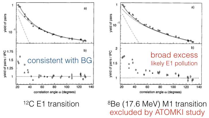
When the Atomki group studied the same 17.64 MeV transition, they found that a key background component—subdominant E1 decays from nearby excited states—dramatically improved the fit and were not included in the original de Boer analysis. This is the last nail in the coffin for the proposed 10 MeV “de Boeron.”

However, the Atomki group also highlight how their new anomaly in the 18.15 MeV state behaves differently. Unlike the broad excess in the de Boer result, the new excess is concentrated in a bump. There is no known way in which additional internal pair creation backgrounds can contribute to add a bump in the opening angle distribution; as noted above: all of these distributions are smoothly falling.

The Atomki group goes on to suggest that the new particle appears to fit the bill for a dark photon, a reasonably well-motivated copy of the ordinary photon that differs in its overall strength and having a non-zero (17 MeV?) mass.

Theory part 1: Not a dark photon

With the Atomki result was published and peer reviewed in Physics Review Letters, the game was afoot for theorists to understand how it would fit into a theoretical framework like the dark photon. A group from UC Irvine, University of Kentucky, and UC Riverside found that actually, dark photons have a hard time fitting the anomaly simultaneously with other experimental constraints. In the visual language of this recent ParticleBite, the situation was this:

Beryllium-8
It turns out that the minimal model of a dark photon cannot simultaneously explain the Atomki beryllium-8 anomaly without running afoul of other experimental constraints. Image adapted from this ParticleBite.

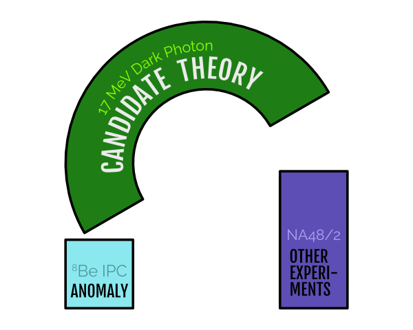
The main reason for this is that a dark photon with mass and interaction strength to fit the beryllium anomaly would necessarily have been seen by the NA48/2 experiment. This experiment looks for dark photons in the decay of neutral pions (π0). These pions typically decay into two photons, but if there’s a 17 MeV dark photon around, some fraction of those decays would go into dark-photon — ordinary-photon pairs. The non-observation of these unique decays rules out the dark photon interpretation.

The theorists then decided to “break” the dark photon theory in order to try to make it fit. They generalized the types of interactions that a new photon-like particle, X, could have, allowing protons, for example, to have completely different charges than electrons rather than having exactly opposite charges. Doing this does gross violence to the theoretical consistency of a theory—but they goal was just to see what a new particle interpretation would have to look like. They found that if a new photon-like particle talked to neutrons but not protons—that is, the new force were protophobic—then a theory might hold together.

Schematic description of how model-builders “hacked” the dark photon theory to fit both the beryllium anomaly while being consistent with other experiments. This hack isn’t pretty—and indeed, comes at the cost of potentially invalidating the mathematical consistency of the theory—but the exercise demonstrates the target for how to a complete theory might have to behave. Image adapted from this ParticleBite.

Theory appendix: pion-phobia is protophobia

Editor’s note: what follows is for readers with some physics background interested in a technical detail; others may skip this section.

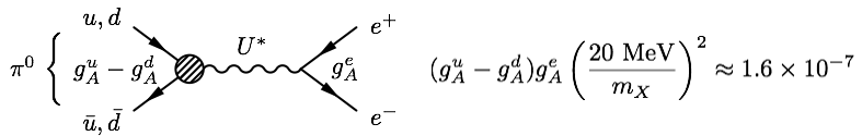
How does a new particle that is allergic to protons avoid the neutral pion decay bounds from NA48/2? Pions decay into pairs of photons through the well-known triangle-diagrams of the axial anomaly. The decay into photon–dark-photon pairs proceed through similar diagrams. The goal is then to make sure that these diagrams cancel.

A cute way to look at this is to assume that at low energies, the relevant particles running in the loop aren’t quarks, but rather nucleons (protons  and neutrons). In fact, since only the proton can talk to the photon, one only needs to consider proton loops. Thus if the new photon-like particle, X, doesn’t talk to protons, then there’s no diagram for the pion to decay into γX. This would be great if the story weren’t completely wrong.

Avoiding NA48
Avoiding NA48/2 bounds requires that the new particle, X, is pion-phobic. It turns out that this is equivalent to X being protophobic. The correct way to see this is on the left, making sure that the contribution of up-quark loops cancels the contribution from down-quark loops. A slick (but naively completely wrong) calculation is on the right, arguing that effectively only protons run in the loop.

The correct way of seeing this is to treat the pion as a quantum superposition of an up–anti-up and down–anti-down bound state, and then make sure that the X charges are such that the contributions of the two states cancel. The resulting charges turn out to be protophobic.

The fact that the “proton-in-the-loop” picture gives the correct charges, however, is no coincidence. Indeed, this was precisely how Jack Steinberger calculated the correct pion decay rate. The key here is whether one treats the quarks/nucleons linearly or non-linearly in chiral perturbation theory. The relation to the Wess-Zumino-Witten term—which is what really encodes the low-energy interaction—is carefully explained in chapter 6a.2 of Georgi’s revised Weak Interactions.

Theory part 2: Not a spin-0 particle

The above considerations focus on a new particle with the same spin and parity as a photon (spin-1, parity odd). Another result of the UCI study was a systematic exploration of other possibilities. They found that the beryllium anomaly could not be consistent with spin-0 particles. For a parity-odd, spin-0 particle, one cannot simultaneously conserve angular momentum and parity in the decay of the excited beryllium-8 state. (Parity violating effects are negligible at these energies.)

Parity
Parity and angular momentum conservation prohibit a “dark Higgs” (parity even scalar) from mediating the anomaly.

For a parity-odd pseudoscalar, the bounds on axion-like particles at 20 MeV suffocate any reasonable coupling. Measured in terms of the pseudoscalar–photon–photon coupling (which has dimensions of inverse GeV), this interaction is ruled out down to the inverse Planck scale.

Screen Shot 2016-08-24 at 4.01.07 PM
Bounds on axion-like particles exclude a 20 MeV pseudoscalar with couplings to photons stronger than the inverse Planck scale. Adapted from 1205.2671 and 1512.03069.

Additional possibilities include:

  • Dark Z bosons, cousins of the dark photon with spin-1 but indeterminate parity. This is very constrained by atomic parity violation.
  • Axial vectors, spin-1 bosons with positive parity. These remain a theoretical possibility, though their unknown nuclear matrix elements make it difficult to write a predictive model. (See section II.D of 1608.03591.)

Theory part 3: Nuclear input

The plot thickens when once also includes results from nuclear theory. Recent results from Saori Pastore, Bob Wiringa, and collaborators point out a very important fact: the 18.15 MeV beryllium-8 state that exhibits the anomaly and the 17.64 MeV state which does not are actually closely related.

Recall (e.g. from the first figure at the top) that both the 18.15 MeV and 17.64 MeV states are both spin-1 and parity-even. They differ in mass and in one other key aspect: the 17.64 MeV state carries isospin charge, while the 18.15 MeV state and ground state do not.

Isospin is the nuclear symmetry that relates protons to neutrons and is tied to electroweak symmetry in the full Standard Model. At nuclear energies, isospin charge is approximately conserved. This brings us to the following puzzle:

If the new particle has mass around 17 MeV, why do we see its effects in the 18.15 MeV state but not the 17.64 MeV state?

Naively, if the new particle emitted, X, carries no isospin charge, then isospin conservation prohibits the decay of the 17.64 MeV state through emission of an X boson. However, the Pastore et al. result tells us that actually, the isospin-neutral and isospin-charged states mix quantum mechanically so that the observed 18.15 and 17.64 MeV states are mixtures of iso-neutral and iso-charged states. In fact, this mixing is actually rather large, with mixing angle of around 10 degrees!

The result of this is that one cannot invoke isospin conservation to explain the non-observation of an anomaly in the 17.64 MeV state. In fact, the only way to avoid this is to assume that the mass of the X particle is on the heavier side of the experimentally allowed range. The rate for emission goes like the 3-momentum cubed (see section II.E of 1608.03591), so a small increase in the mass can suppresses the rate of emission by the lighter state by a lot.

The UCI collaboration of theorists went further and extended the Pastore et al. analysis to include a phenomenological parameterization of explicit isospin violation. Independent of the Atomki anomaly, they found that including isospin violation improved the fit for the 18.15 MeV and 17.64 MeV electromagnetic decay widths within the Pastore et al. formalism. The results of including all of the isospin effects end up changing the particle physics story of the Atomki anomaly significantly:

Parameter fits
The rate of X emission (colored contours) as a function of the X particle’s couplings to protons (horizontal axis) versus neutrons (vertical axis). The best fit for a 16.7 MeV new particle is the dashed line in the teal region. The vertical band is the region allowed by the NA48/2 experiment. Solid lines show the dark photon and protophobic limits. Left: the case for perfect (unrealistic) isospin. Right: the case when isospin mixing and explicit violation are included. Observe that incorporating realistic isospin happens to have only a modest effect in the protophobic region. Figure from 1608.03591.

The results of the nuclear analysis are thus that:

  1. An interpretation of the Atomki anomaly in terms of a new particle tends to push for a slightly heavier X mass than the reported best fit. (Remark: the Atomki paper does not do a combined fit for the mass and coupling nor does it report the difficult-to-quantify systematic errors  associated with the fit. This information is important for understanding the extent to which the X mass can be pushed to be heavier.)
  2. The effects of isospin mixing and violation are important to include; especially as one drifts away from the purely protophobic limit.

Theory part 4: towards a complete theory

The theoretical structure presented above gives a framework to do phenomenology: fitting the observed anomaly to a particle physics model and then comparing that model to other experiments. This, however, doesn’t guarantee that a nice—or even self-consistent—theory exists that can stretch over the scaffolding.

Indeed, a few challenges appear:

  • The isospin mixing discussed above means the X mass must be pushed to the heavier values allowed by the Atomki observation.
  • The “protophobic” limit is not obviously anomaly-free: simply asserting that known particles have arbitrary charges does not generically produce a mathematically self-consistent theory.
  • Atomic parity violation constraints require that the X couple in the same way to left-handed and right-handed matter. The left-handed coupling implies that X must also talk to neutrinos: these open up new experimental constraints.

The Irvine/Kentucky/Riverside collaboration first note the need for a careful experimental analysis of the actual mass ranges allowed by the Atomki observation, treating the new particle mass and coupling as simultaneously free parameters in the fit.

Next, they observe that protophobic couplings can be relatively natural. Indeed: the Standard Model Z boson is approximately protophobic at low energies—a fact well known to those hunting for dark matter with direct detection experiments. For exotic new physics, one can engineer protophobia through a phenomenon called kinetic mixing where two force particles mix into one another. A tuned admixture of electric charge and baryon number, (Q-B), is protophobic.

Baryon number, however, is an anomalous global symmetry—this means that one has to work hard to make a baryon-boson that mixes with the photon (see 1304.0576 and 1409.8165 for examples). Another alternative is if the photon kinetically mixes with not baryon number, but the anomaly-free combination of “baryon-minus-lepton number,” Q-(B-L). This then forces one to apply additional model-building modules to deal with the neutrino interactions that come along with this scenario.

In the language of the ‘model building blocks’ above, result of this process looks schematically like this:

Model building block
A complete theory is completely mathematically self-consistent and satisfies existing constraints. The additional bells and whistles required for consistency make additional predictions for experimental searches. Pieces of the theory can sometimes  be used to address other anomalies.

The theory collaboration presented examples of the two cases, and point out how the additional ‘bells and whistles’ required may tie to additional experimental handles to test these hypotheses. These are simple existence proofs for how complete models may be constructed.

What’s next?

We have delved rather deeply into the theoretical considerations of the Atomki anomaly. The analysis revealed some unexpected features with the types of new particles that could explain the anomaly (dark photon-like, but not exactly a dark photon), the role of nuclear effects (isospin mixing and breaking), and the kinds of features a complete theory needs to have to fit everything (be careful with anomalies and neutrinos). The single most important next step, however, is and has always been experimental verification of the result.

While the Atomki experiment continues to run with an upgraded detector, what’s really exciting is that a swath of experiments that are either ongoing or in construction will be able to probe the exact interactions required by the new particle interpretation of the anomaly. This means that the result can be independently verified or excluded within a few years. A selection of upcoming experiments is highlighted in section IX of 1608.03591:

Experimental searches
Other experiments that can probe the new particle interpretation of the Atomki anomaly. The horizontal axis is the new particle mass, the vertical axis is its coupling to electrons (normalized to the electric charge). The dark blue band is the target region for the Atomki anomaly. Figure from 1608.03591; assuming 100% branching ratio to electrons.

We highlight one particularly interesting search: recently a joint team of theorists and experimentalists at MIT proposed a way for the LHCb experiment to search for dark photon-like particles with masses and interaction strengths that were previously unexplored. The proposal makes use of the LHCb’s ability to pinpoint the production position of charged particle pairs and the copious amounts of D mesons produced at Run 3 of the LHC. As seen in the figure above, the LHCb reach with this search thoroughly covers the Atomki anomaly region.

Implications

So where we stand is this:

  • There is an unexpected result in a nuclear experiment that may be interpreted as a sign for new physics.
  • The next steps in this story are independent experimental cross-checks; the threshold for a ‘discovery’ is if another experiment can verify these results.
  • Meanwhile, a theoretical framework for understanding the results in terms of a new particle has been built and is ready-and-waiting. Some of the results of this analysis are important for faithful interpretation of the experimental results.

What if it’s nothing?

This is the conservative take—and indeed, we may well find that in a few years, the possibility that Atomki was observing a new particle will be completely dead. Or perhaps a source of systematic error will be identified and the bump will go away. That’s part of doing science.

Meanwhile, there are some important take-aways in this scenario. First is the reminder that the search for light, weakly coupled particles is an important frontier in particle physics. Second, for this particular anomaly, there are some neat take aways such as a demonstration of how effective field theory can be applied to nuclear physics (see e.g. chapter 3.1.2 of the new book by Petrov and Blechman) and how tweaking our models of new particles can avoid troublesome experimental bounds. Finally, it’s a nice example of how particle physics and nuclear physics are not-too-distant cousins and how progress can be made in particle–nuclear collaborations—one of the Irvine group authors (Susan Gardner) is a bona fide nuclear theorist who was on sabbatical from the University of Kentucky.

What if it’s real?

This is a big “what if.” On the other hand, a 6.8σ effect is not a statistical fluctuation and there is no known nuclear physics to produce a new-particle-like bump given the analysis presented by the Atomki experimentalists.

The threshold for “real” is independent verification. If other experiments can confirm the anomaly, then this could be a huge step in our quest to go beyond the Standard Model. While this type of particle is unlikely to help with the Hierarchy problem of the Higgs mass, it could be a sign for other kinds of new physics. One example is the grand unification of the electroweak and strong forces; some of the ways in which these forces unify imply the existence of an additional force particle that may be light and may even have the types of couplings suggested by the anomaly.

Could it be related to other anomalies?

The Atomki anomaly isn’t the first particle physics curiosity to show up at the MeV scale. While none of these other anomalies are necessarily related to the type of particle required for the Atomki result (they may not even be compatible!), it is helpful to remember that the MeV scale may still have surprises in store for us.

  • The KTeV anomaly: The rate at which neutral pions decay into electron–positron pairs appears to be off from the expectations based on chiral perturbation theory. In 0712.0007, a group of theorists found that this discrepancy could be fit to a new particle with axial couplings. If one fixes the mass of the proposed particle to be 20 MeV, the resulting couplings happen to be in the same ballpark as those required for the Atomki anomaly. The important caveat here is that parameters for an axial vector to fit the Atomki anomaly are unknown, and mixed vector–axial states are severely constrained by atomic parity violation.
KTeV anomaly
The KTeV anomaly interpreted as a new particle, U. From 0712.0007.
  • The anomalous magnetic moment of the muon and the cosmic lithium problem: much of the progress in the field of light, weakly coupled forces comes from Maxim Pospelov. The anomalous magnetic moment of the muon, (g-2)μ, has a long-standing discrepancy from the Standard Model (see e.g. this blog post). While this may come from an error in the very, very intricate calculation and the subtle ways in which experimental data feed into it, Pospelov (and also Fayet) noted that the shift may come from a light (in the 10s of MeV range!), weakly coupled new particle like a dark photon. Similarly, Pospelov and collaborators showed that a new light particle in the 1-20 MeV range may help explain another longstanding mystery: the surprising lack of lithium in the universe (APS Physics synopsis).

Could it be related to dark matter?

A lot of recent progress in dark matter has revolved around the possibility that in addition to dark matter, there may be additional light particles that mediate interactions between dark matter and the Standard Model. If these particles are light enough, they can change the way that we expect to find dark matter in sometimes surprising ways. One interesting avenue is called self-interacting dark matter and is based on the observation that these light force carriers can deform the dark matter distribution in galaxies in ways that seem to fit astronomical observations. A 20 MeV dark photon-like particle even fits the profile of what’s required by the self-interacting dark matter paradigm, though it is very difficult to make such a particle consistent with both the Atomki anomaly and the constraints from direct detection.

Should I be excited?

Given all of the caveats listed above, some feel that it is too early to be in “drop everything, this is new physics” mode. Others may take this as a hint that’s worth exploring further—as has been done for many anomalies in the recent past. For researchers, it is prudent to be cautious, and it is paramount to be careful; but so long as one does both, then being excited about a new possibility is part what makes our job fun.

For the general public, the tentative hopes of new physics that pop up—whether it’s the Atomki anomaly, or the 750 GeV diphoton bumpa GeV bump from the galactic center, γ-ray lines at 3.5 keV and 130 GeV, or penguins at LHCb—these are the signs that we’re making use of all of the data available to search for new physics. Sometimes these hopes fizzle away, often they leave behind useful lessons about physics and directions forward. Maybe one of these days an anomaly will stick and show us the way forward.

Further Reading

Here are some of the popular-level press on the Atomki result. See the references at the top of this ParticleBite for references to the primary literature.

UC Riverside Press Release
UC Irvine Press Release
Nature News
Quanta Magazine
Quanta Magazine: Abstractions
Symmetry Magazine
Los Angeles Times

What is “Model Building”?

One thing that makes physics, and especially particle physics, is unique in the sciences is the split between theory and experiment. The role of experimentalists is clear: they build and conduct experiments, take data and analyze it using mathematical, statistical, and numerical techniques to separate signal from background. In short, they seem to do all of the real science!

So what is it that theorists do, besides sipping espresso and scribbling on chalk boards? In this post we describe one type of theoretical work called model building. This usually falls under the umbrella of phenomenology, which in physics refers to making connections between mathematically defined theories (or models) of nature and actual experimental observations of nature.

One common scenario is that one experiment observes something unusual: an anomaly. Two things immediately happen:

  1. Other experiments find ways to cross-check to see if they can confirm the anomaly.
  2. Theorists start figure out the broader implications if the anomaly is real.

#1 is the key step in the scientific method, but in this post we’ll illuminate what #2 actually entails. The scenario looks a little like this:

An unusual experimental result (anomaly) is observed. Is it consistent with other experimental observations?
An unusual experimental result (anomaly) is observed. One thing we would like to know is whether it is consistent with other experimental observations, but these other observations may not be simply related to the anomaly.

Theorists, who have spent plenty of time mulling over the open questions in physics, are ready to apply their favorite models of new physics to see if they fit. These are the models that they know lead to elegant mathematical results, like grand unification or a solution to the Hierarchy problem. Sometimes theorists are more utilitarian, and start with “do it all” Swiss army knife theories called effective theories (or simplified models) and see if they can explain the anomaly in the context of existing constraints.

Here’s what usually happens:

Usually the nicest models of new physics don't fit.
Usually the nicest models of new physics don’t fit! In the explicit example, the minimal supersymmetric Standard Model doesn’t include a good candidate to explain the 750 GeV diphoton bump.

Indeed, usually one needs to get creative and modify the nice-and-elegant theory to make sure it can explain the anomaly while avoiding other experimental constraints. This makes the theory a little less elegant, but sometimes nature isn’t elegant.

Candidate theory extended with a module (in this case, an additional particle). This additional model is “bolted on” to the theory to make it fit the experimental observations.

Now we’re feeling pretty good about ourselves. It can take quite a bit of work to hack the well-motivated original theory in a way that both explains the anomaly and avoids all other known experimental observations. A good theory can do a couple of other things:

  1. It points the way to future experiments that can test it.
  2. It can use the additional structure to explain other anomalies.

The picture for #2 is as follows:

A good hack to a theory can explain multiple anomalies.
A good hack to a theory can explain multiple anomalies. Sometimes that makes the hack a little more cumbersome. Physicists often develop their own sense of ‘taste’ for when a module is elegant enough.

Even at this stage, there can be a lot of really neat physics to be learned. Model-builders can develop a reputation for particularly clever, minimal, or inspired modules. If a module is really successful, then people will start to think about it as part of a pre-packaged deal:

A really successful hack may eventually be added to the list of candidate theories.
A really successful hack may eventually be thought of as it’s own variant of the original theory.

Model-smithing is a craft that blends together a lot of the fun of understanding how physics works—which bits of common wisdom can be bent or broken to accommodate an unexpected experimental result? Is it possible to find a simpler theory that can explain more observations? Are the observations pointing to an even deeper guiding principle?

Of course—we should also say that sometimes, while theorists are having fun developing their favorite models, other experimentalists have gone on to refute the original anomaly.

Sometimes anomalies go away.
Sometimes anomalies go away and the models built to explain them don’t hold together.

But here’s the mark of a really, really good model: even if the anomaly goes away and the particular model falls out of favor, a good model will have taught other physicists something really neat about what can be done within the a given theoretical framework. Physicists get a feel for the kinds of modules that are out in the market (like an app store) and they develop a library of tricks to attack future anomalies. And if one is really fortunate, these insights can point the way to even bigger connections between physical principles.

I cannot help but end this post without one of my favorite physics jokes, courtesy of T. Tait:

A theorist and an experimentalist are having coffee. The theorist is really excited, she tells the experimentalist, “I’ve got it—it’s a model that’s elegant, explains everything, and it’s completely predictive.”

The experimentalist listens to her colleague’s idea and realizes how to test those predictions. She writes several grant applications, hires a team of postdocs and graduate students, trains them,  and builds the new experiment. After years of design, labor, and testing, the machine is ready to take data. They run for several months, and the experimentalist pores over the results.

The experimentalist knocks on the theorist’s door the next day and says, “I’m sorry—the experiment doesn’t find what you were predicting. The theory is dead.”

The theorist frowns a bit: “What a shame. Did you know I spent three whole weeks of my life writing that paper?”

Respecting your “Elders”

Theoretical physicists have designed a new way to explain the how dark matter interactions can explain the observed amount of dark matter in the universe today. This elastically decoupling dark matter framework, is a hybrid of conventional and novel dark matter models.

Presenting: Elastically Decoupling Dark Matter
Authors: Eric Kuflik, Maxim Perelstein, Nicolas Rey-Le Lorier, Yu-Dai Tsai
Reference: 1512.04545, Phys. Rev. Lett. 116, 221302 (2016)

The particle identity of dark matter is one of the biggest open questions in physics. The simplest and most widely assumed explanation is that dark matter is a weakly-interacting massive particle (WIMP). Assuming that dark matter starts out in thermal equilibrium in the hot plasma of the early universe, the present cosmic abundance of WIMPs is set by the balance of two effects:

  1. When two WIMPs find each other, they can annihilate into ordinary matter. This depletes the number of WIMPs in the universe.
  2. The universe is expanding, making it harder for WIMPs to find each other.

This process of “thermal freeze out” leads to an abundance of WIMPs controlled by the dark matter mass and interaction strength. The term ‘weakly-interacting massive particle’ comes from the observation that dark matter of roughly the mass of the weak force particle that interact through the weak nuclear force gives the experimentally measured dark matter density today.

Two ways for a new particle, X, to produce the observed dark matter abundance: (left) conventional WIMP annihilation into Standard Model (SM) particles versus (right) strongly-Interacting 3-to-2 interactions that reduce the amount of dark matter.
Two ways for a new particle, X, to produce the observed dark matter abundance: (left) WIMP annihilation into Standard Model (SM) particles versus (right) SIMP 3-to-2 interactions that reduce the amount of dark matter.

More recently, physicists noticed that dark matter with very large interactions with itself (not ordinary matter), can produce the correct dark matter density in another way. These “strongly interacting massive particle” models reduce regulate the amount of dark matter through 3-to-2 interactions that reduce the total number of dark matter particles rather than annihilation into ordinary matter.

The authors of 1512.04545 have proposed an intermediate road that interpolates between these two types of dark matter. The “elastically decoupling dark matter” (ELDER) scenario. ELDERs have both of the above interactions: they can annihilate pairwise into ordinary matter, or sets of three ELDERs can turn into two ELDERS.

ELDER scenario
Thermal history of ELDERs, adapted from 1512.04545.

The cosmic history of these ELDERs is as follows:

  1. ELDERs are produced in thermal bath immediately after the big bang.
  2. Pairs of ELDERS annihilate into ordinary matter. Like WIMPs, they interact weakly with ordinary matter.
  3. As the universe expands, the rate for annihilation into Standard Model particles falls below the rate at which the universe expands
  4. Assuming that the ELDERs interact strongly amongst themselves, the 3-to-2 number-changing process still occurs. Because this process distributes the energy of 3 ELDERs in the initial state to 2 ELDERs in the final state, the two outgoing ELDERs have more kinetic energy: they’re hotter. This turns out to largely counteract the effect of the expansion of the universe.

The neat effect here is the abundance of ELDERs is actually set by the interaction with ordinary matter, like WIMPs. However, because they have this 3-to-2 heating period, they are able to produce the observed present-day dark matter density for very different choices of interactions. In this sense, the authors show that this framework opens up a new “phase diagram” in the space of dark matter theories:

A "phase diagram" of dark matter models. The vertical axis represents the dark matter self-coupling strength while the horizontal axis represents the coupling to ordinary matter.
A “phase diagram” of dark matter models. The vertical axis represents the dark matter self-coupling strength while the horizontal axis represents the coupling to ordinary matter.

Background reading on dark matter:

What Scientists Should Know About Science Hack Day

One of the failures of conventional science outreach is that it’s easy to say what our science is about, but it’s very difficult to convey what it’s like to do science. And on top of that, how can we do this in a way that:

  • scales and can be ported to different places
  • generates and nurtures a continued interest in science
  • can patch on to practical and useful citizen science
  • requires only a modest input from specialists?

Well, now there’s a killer-app for that.


Science Hack Day: San Francisco

I recently had the distinct privilege of participating in this year’s Science Hack Day (SHD) in San Francisco as a Science Ambassador. On the surface, SHD is a science-themed hackathon: a weekend where people get together to collaboratively develop on neat ideas. More than this, though, Science Hack Day encapsulates precisely the joy of collaborative discovery and problem solving that drew me into a career in research.

Massively Multiplayer Science
Ariel Waldman, ‘global instigator’ for Science Hack Day, gives the open remarks at Science Hack Day: SF.

I cannot understate how much this resonated with me as a scientist: over the course of about 30 hours, SHD was able to create a microcosm of how we do science, and it was able to do so in a way that brought together people of very different age groups, genders, ethnicities, and professional backgrounds to hack and learn and create. Many of these projects made use of open data sets, and many of them ended up open source: either in the form of GitHub repositories for software or instructables for more physical creations.

The hacks ranged from fun— such as a board game based on the immune system, to practical—a Chrome app that overlays CO2 emissions onto Google Maps. They were marketable—a 3D candy pen, and mesmerizing—an animation of 15 years of hand-drawn solar records. Some were simply inspiring, such as coordinating a day to view the rings of saturn to spark interest in science.

The Best Parts of Grad School in 30 Hours

One thing that especially rang true to me was that Science Hack Day—like the actual day-to-day science done by researchers—is not about deliverables. The science isn’t the poster that you glued together at your 4th grade science fair (or the journal article that is similarly glued together decades later), it’s all of the action before that. It’s about casual brainstorming, “literature reviews” looking for existing off-the-shelf tools, bumping into experts and getting their feedback, the many times things break—and the breakthroughs from understanding why, and then the devil-may-care kludges to get a prototype up and running with your teammates.

All that is what I want to convey when people tell me that particle physics sounds neat, but what exactly is it that we do all day long in the ivory tower? Now I know the answer: we’re science hacking—and you can try it out, too.

DSC02999
Ariel’s tips for Science Hack Day are also useful reminders for academic researchers… and really, probably for everyone.

And this, if you ask me, is precisely what needs to be injected into science outreach. It’s always fantastic when people are wow’ed by inspiring talks by charismatic scientists—but nothing can replace the pure joy of actually putting on the proverbial lab coat and losing yourself in curiosity-based tinkering and problem solving.

Boots on the ground outreach

I owe a lot to Matt Bellis, a physicist and SHD veteran, for preparing me for SHD. He describes the event from the point of view of a scientist as “boots on the ground outreach.” Science Hack Day is a way to “engage” with the science-minded public in a meaningful way.

And by “engage” I mean “make cool things.” I also mean “interact with as colleagues rather than as a teacher.”

And by “science-minded public,” I really mean a slice of the public are already interested in science, but are also interested in participating as citizen scientists, continuing to tinker with code on GitHub or even just spreading the joy of science-themed hacking to their respective communities. This is science wanting to go viral, and the SHD participants want to be patient zeroes.

Image courtesy of Matt Biddulph.
A shot of the crowd before project presentations at SHD:SF 2015. Image courtesy of Matt Biddulph.

SHD is free, volunteer driven (an Avogadro’s number of thank yous to the SHD organizers and volunteers), and open to the community. The demographics of the crowd at SHD:SF was a lot closer to the actual population of San Francisco, and is thus a lot closer to the demographics that we academics want to also see reflected in the academy. Events like SHD aren’t just preaching to the choir, it’s a real opportunity to promote STEM fields broadly to underrepresented groups.

In fact, think about the moment that you were hooked on science. For many of us, those moments are a combination of serendipity and opportunity. What would it take to bring that to make that spark accessible? SHD is one such event. And in fact, it even generated a science hack for precisely that.

Open Science

There was also a valuable message to glean from the crowd at the event: people want to play with data. And for the general public, they’re even happier when academics provide tools to play with data.

Data doesn’t even have to be what you conventionally think of as data. Alex Parker’s “solar archive” won the “best use of data” award for a dataset of 15 years of daily hand drawn images of the sun by astronomers at the Mount Wilson Observatory. Alex’s team used image processing techniques to clean, organize, and animate the images. The result is hypnotic to watch, but is also a gateway to actual science education: what are these sun spots that they’re annotating? How did they draw these images? What can we learn from this record?

opensciencehack
Giving a “lightning talk” on data sets in particle physics. Slides available.

Open data sets are a little more difficult in particle physics: collider data is notoriously subtle to perform analyses—mostly because background subtraction typically requires advanced physics background. Nevertheless, our field is evolving slowly and there are now some options available. See my lightning talk slides for a brief discussion of these with links.

The point, though, is that there is demand. And for the public, the more people demand open data sets—even just for “playing”—the more scientists will understand the potential for productive partnerships with citizen scientists. And for scientists: make your tools available. This holds true even for technical tools—GitHub is a great way to get your colleagues to pick up the research directions you find exciting by sharing Mathematica or Jupyter notebooks!


The Science Hack Day Movement

SHD San Francisco participants video chatted with participants from parallel SHD events going on in Berlin and Madagascar. Photo courtesy of Matt Biddulph.
SHD San Francisco participants were able to video chat with participants from parallel SHD events going on in Berlin and Madagascar. Photo courtesy of Matt Biddulph.

A quick look at the SHD main page shows that Science Hack Days are popping up all over the world. In true open source spirit, SHD even has a set of resources for putting together your own Science Hack Day event. In other words, Science Hack Day scales—you can build upon the experiences of past events to build your own. I suspect that there is untapped potential to seed Science Hack Day into universities, where many computer science departments have experience with hackathons and many physics departments have a large set of lecture demonstrations that may be amenable to hacking.

Needless to say, the weekend turned me into a Science Hack Day believer. I strongly encourage anyone of any scientific background to try out one of these events: it’s a weekend that doesn’t require any advance planning (though it helps to brainstorm), and you’ll be surprised at neat things you can develop, and what neat new friends you make along the way. And that, to me, is a summary of what’s great about doing science.

See you at the next Science Hack Day!


Many thanks to the people who made SHD:SF so magical for me: Jun Axup and Rose Broome for delightful conversations and their enthusiasm, Matt Biddulph for taking photos, Mayank Kedia, Kris Kooi, and Chrisantha Perera for hacking with me, all of the volunteers and sponsors (especially the Sloan and Moore foundations for supporting the ambassador program), Matt Bellis for passing on his past projects and data sets, and all of the wonderful hackers who I got to learn from and chat with. Most importantly, though, huge thanks and gratitude to Ariel Waldman, who is the driving force of the Science Hack Day movement and has brought so much joy and science to so many people while simultaneously being incredibly modest about her contributions. 

Dark Photons from the Center of the Earth

Presenting: Dark Photons from the Center of the Earth
Author: J. Feng, J. Smolinsky, P. Tanedo (disclosure: blog post is by an author on the paper)
Reference: arXiv:1509.07525

Dark matter may be collecting in the center of the Earth. A recent paper explores way to detect its decay products here on the surface.

Dark matter may collect in the Earth and annihilate in to dark photons, which propagate to the surface before decaying into pairs of particles that can be detected by IceCube.
Dark matter may collect in the Earth and annihilate in to dark photons, which propagate to the surface before decaying into pairs of particles that can be detected by a large-volume neutrino detector like IceCube. Image from arXiv:1509.07525.

Our entire galaxy is gravitationally held together by a halo of dark matter, whose particle properties remain one of the biggest open questions in high energy physics. One class of theories assumes that the dark matter particles interact through a dark photon, a hypothetical particle which mediates a force analogous to how the ordinary photon mediates electromagnetism.

These theories also permit the  ordinary and dark photons to have a small quantum mechanical mixing. This effectively means that the dark photon can interact very weakly with ordinary matter and mediate interactions between ordinary matter and dark matter—this gives a handle for ways to detect dark matter.

While most methods for detecting dark matter focus on building detectors that are sensitive to the “wind” of dark matter bombarding (and mostly passing through) the Earth as the solar system zooms through the galaxy, the authors of 1509.07525 follow up on an idea initially proposed in the mid-80’s: dark matter hitting the Earth might get stuck in the Earth’s gravitational potential and build up in its core.

These dark matter particles can then find each other and annihilate. If they annihilate into very weakly interacting particles, then these may be detected at the surface of the Earth. A typical example is dark matter annihilation into neutrinos. In 1509.07525, the authors examine the case where the dark matter annihilates into dark photons, which can pass through the Earth as easily as a neutrino and decay into pairs of electrons or muons near the surface.

These decays can be detected in large neutrino detectors, such as the IceCube neutrino observatory (previously featured in ParticleBites). In the case where the dark matter is very heavy (e.g. TeV in mass) and the dark photons are very light (e.g. 200 MeV), these dark photons are very boosted and their decay products point back to the center of the Earth. This is a powerful discriminating feature against background cosmic ray events.  The number of signal events expected is shown in the following contour plot:

Number of signal (Nsig) dark photon decays expected at the IceCube detector in the plane of dark photon mixing over dark photon mass.
Number of signal dark photon decays expected at the IceCube detector in the plane of dark photon mixing over dark photon mass. Image from arXiv 1509.07525. Blue region is in tension with direct detection bounds (from ariv:1507.04007), while the gray regions are in tension with beam dump and supernovae bounds, see e.g. arXiv:1311.029.

While similar analyses for dark photon-mediated dark matter capture by celestial bodies and annihilation have been studied—see e.g. Pospelov et al., Delaunay et al., Schuster et al., and Meade et al.—the authors of 1509.07525 focus on the case of dark matter capture in the Earth (rather than, say, the sun) and subsequent annihilation to dark photons (rather than neutrinos).

  1. The annihilation rate at the center of the Earth is greatly increased do to Sommerfeld enhancement: because the captured dark matter has very low velocity, it is much more likely to annihilate with other captured dark matter particles due to mutual attraction from dark photon exchange.
  2. This causes the Earth to quickly saturate with dark matter, leading to larger annihilation rates than one would naively expect in the case where the Earth were not yet dark matter saturated such that annihilation and capture occur at equal rates.
  3. In addition using directional information to identify signal events against cosmic ray backgrounds, the authors identified kinematic quantities—the opening angle of the Standard Model decay products and the time delay between them—as ways to further discriminate signal from background. Unfortunately their analysis implies that these features lie just outside of the IceCube sensitivity to them.

Finally, the authors point out the possibility of large enhancements coming from the so-called dark disk, an enhancement in the low velocity phase space density of dark matter. If that is the case, then the estimated reach may increase by an order of magnitude.


Suggested further reading:

How much top quark is in the proton?

We know that protons are made up of two up quarks and a down quark. Each only weigh a few MeV—the rest of the proton mass comes from the strong force binding energy coming from gluon exchange. When we collider protons at high energies, these partons interact with each other to produce other particles. In fact, the LHC is essentially a gluon collider. Recently, however, physicists have been asking, “How much top quark is there in the proton?

Presenting: Top-Quark Initiated Processes at High-Energy Hadron Colliders
Authors: Tao Han, Joshua Sayre, Susanne Westhoff (Pittsburgh U.)
Reference: 1411.2588JHEP 1504 (2015) 145

In fact, at first glance, this is a ridiculous question. The top quark is 175 times heavier than the proton! How does it make sense that there are top quarks “in” the proton?

The proton (1 GeV mass) doesn't seem to have room for any top quark component (175 GeV mass).
The proton (1 GeV mass) doesn’t seem to have room for any top quark component (175 GeV mass).

The discussion is based on preliminary plans to build a 100 TeV collider, though there’s a similar story for b quarks (5 times the mass of the proton) at the LHC.

Before we define what we mean by treating the top as a parton, we should define what we mean by proton! We can describe the proton constituents by a series of parton distribution functions (pdf): these tell us the probability of that you’ll interact with a particular piece of the proton. These pdfs are energy-dependent: at high energies, it turns out that you’re more likely to interact with a gluon than any of the “valence quarks.” At sufficiently high energies, these gluons can also produce pairs of heavier objects, like charm, bottom, and—at 100 TeV—even top quarks.

But there’s an even deeper sense in which these heavy quarks have a non-zero parton distribution function (i.e. “fraction of the proton”): it turns out that perturbation theory breaks down for certain kinematic regions when a gluon splits into quarks. That is to say, the small parameters we usually expand in become large.

Theoretically, a technique to keep the expansion parameter small leads to an interpretation of this “high-energy gluon splitting into heavy quarks inside the proton” process as the proton having some intrinsic heavy quark content. This is called perturbative QCD, the key equation known as DGLAP.

High energy gluon splittings can yield top quarks (lines with arrows). When one of these top quarks is collinear with the beam (pink, dashed), the calculation becomes non-perturbative.
High energy gluon splittings can yield top quarks (lines with arrows). When one of these top quarks is collinear with the beam (pink, dashed), the calculation becomes non-perturbative. Maintaining the perturbation expansion parameter leads on to treat the top quark as a constituent of the proton. Solid blue lines are not-collinear and are well-behaved.

In the cartoon above: physically what’s happening is that a gluon in the proton splits into a top and anti-top. When one of these is collinear (i.e. goes down the collider beamline), the expansion parameter blows up and the calculation misbehaves. In order to maintain a well behaved perturbation theory, DGLAP tells us to pretend that instead of a top/anti-top pair coming from a gluon splitting, one can treat these as a top that lives inside the high-energy proton.

A gluon splitting that gives a non-perturvative top can be treated as a top inside the proton.

This is the sense in which the top quark can be considered as a parton. It doesn’t have to do with whether the top “fits” inside a proton and whether this makes sense given the mass—it boils down to a trick to preserve perturbativity.

One can recast this as the statement that the proton (or even fundamental particles like the electron) look different when you probe them at different energy scales. One can compare this story to this explanation for why the electron doesn’t have infinite electromagnetic energy.

The authors of 1411.2588 a study of the sensitivity a 100 TeV collider to processes that are produced from fusion of top quarks “in” each proton. With any luck, such a collider may even be on the horizon for future generations.

A Tau Neutrino Runs into a Candy Shop…

We recently discussed some curiosities in the data from the IceCube neutrino detector. This is a follow up Particle Bite on some of the sugary nomenclature IceCube uses to characterize some of its events.

As we explained previously, IceCube is a gigantic ultra-high energy cosmic neutrino detector in Antarctica. These neutrinos have energies between 10-100 times higher than the protons colliding at the Large Hadron Collider, and their origin and nature are largely a mystery. One thing that IceCube can tell us about these neutrinos is their flavor composition; see e.g. this post for a crash course in neutrino flavor.

When neutrinos interact with ambient nuclei through a W boson (charged current interactions), the following types of events might be seen:

Types of Ice Cube Events
Typical charged current events in IceCube. Displays from the IceCube collaboration.

I refer you to this series of posts for a gentle introduction to the Feynman diagrams above. The key is that the high energy neutrino interacts with an nucleus, breaking it apart (the remnants are called X above) and ejecting a high energy charged lepton which can be used to identify the flavor of the neutrino.

  • Muons travel a long distance and leave behind a trail of Cerenkov radiation called a track.
  • Electrons don’t travel as far and deposit all of their energy into a shower. These are also sometimes called cascades because of the chain of particles produced in the ‘bang’.
  • Taus typically leave a more dramatic signal, a double bang, when the tau is formed and then subsequently decays into more hadrons (X’ above).

In fact, the tau events can be further classified depending on how this ‘double bang’ is resolved—and it seems like someone was playing a popular candy-themed mobile game when naming these:

Types of tau events in IceCube from Cowan.
Types of candy-themed tau events in IceCube from D. Cowan at the TeVPA 2 conference.

In this figure from the TeVPA 2 conference proceedings, we find some silly classifications of what tau events look like according to their energy:

  • Lollipop: The tau is produced outside the detector so that the first ‘bang’ isn’t seen. Instead, there’s a visible track that leads to the second (observable) bang. The track is the stick and the bang is the lollipop head.
  • Inverted lollipop: Similar to the lollipop, except now the first ‘bang’ is seen in the detector but the second ‘bang’ occurs outside the detector and is not observed.
  • Sugardaddy: The tau is produced outside the detector but decays into a muon inside the detector. This looks almost like a muon track except that the tau produces less Cerenkov light so that one can identify the point where the tau decays into a muon.
  • Double pulse: While this isn’t candy-themed, it’s still very interesting. This is a double bang where the two bangs can’t be distinguished spatially. However, since one bang occurs slightly after the other, one can distinguish them in the time: it’s a “double bang” in time rather than space.
  • Tautsie pop: This is a low energy version of the sugardaddy where the shower-to-track energy is used to discriminate against background.

While the names may be silly, counting these types of events in IceCube is one of the exciting frontiers of flavor physics. And while we might be forgiven for thinking that neutrino physics is all about measuring very `small’ things—let me share the following graphic from Francis Halzen’s recent talk at the AMS Days workshop at CERN, overlaying one of the shower events over Madison, Wisconsin to give a sense of scale:

From F. Halzen on behalf of the IceCube collaboration.
From F. Halzen on behalf of the IceCube collaboration; from AMS Days at CERN 2015.

The Glashow Resonance on Ice

Are cosmic neutrinos trying to tell us something, deep in the Antarctic ice?

Presenting:

“Glashow resonance as a window into cosmic neutrino sources,”
by Barger, Lu, Learned, Marfatia, Pakvasa, and Weiler
Phys.Rev. D90 (2014) 121301 [1407.3255]

Related work: Anchordoqui et al. [1404.0622], Learned and Weiler [1407.0739], Ibe and Kaneta [1407.2848]

Is there an neutrino energy cutoff preventing Glashow resonance events in IceCube?

The IceCube Neutrino Observatory is a gigantic neutrino detector located in the Antarctic. Like an iceberg, only a small fraction of the lab is above ground: 86 strings extend to a depth of 2.5 kilometers into the ice, with each string instrumented with 60 detectors.

2 PeV event from the IceCube 3 year analysis; nicknamed "Big Bird." From 1405.5303.
2 PeV event from the IceCube 3 year analysis; nicknamed “Big Bird.” From 1405.5303.

These detectors search ultra high energy neutrinos by looking for Cerenkov radiation as they pass through the ice. This is really the optical version of a sonic boom. An example event is shown above, where the color and size of the spheres indicate the strength of the Cerenkov signal in each detector.

IceCube has released data for its first three years of running (1405.5303) and has found three events with very large energies: 1-2 peta-electron-volts: that’s ten thousand times the mass of the Higgs boson. In addition, there’s a spectrum of neutrinos in the 10-1000 TeV range.

Glashow resonance diagram.

These ultra high energy neutrinos are believed to originate from outside our galaxy through processes involving particle acceleration by black holes. One expects the flux of such neutrinos to go as a power law of the energy, \Phi \sim E^{-\alpha} where \alpha = 2 is a estimate from certain acceleration models. The existence of the three super high energy events at the PeV scale has led some people to think about a known deviation from the power law spectrum: the Glashow resonance. This is the sharp increase in the rate of neutrino interactions with matter coming from the resonant production of W bosons, as shown in the Feynman diagram to the left.

The Glashow resonance sticks out like a sore thumb in the spectrum. The position of the resonance is set by the energy required for an electron anti-neutrino to hit an electron at rest such that the center of mass energy is the W boson mass.

astro-ph/0101216
Sharp peak in the neutrino scattering rate from the Glashow resonance; image from Engel, Seckel, and Stanev in astro-ph/0101216.

If you work through the math on the back of an envelope, you’ll find that the resonance occurs for incident electron anti-neutrinos with an energy of  6.3 PeV; see figure to the leftt. This is “right around the corner” from the 1-2 PeV events already seen, and one might wonder whether it’s significant that we haven’t seen anything.

The authors of [1407.3255] have found that the absence of Glashow resonant neutrino events in IceCube is not yet a bona-fide “anomaly.” In fact, they point out that the future observation or non-observation of such neutrinos can give us valuable hints about the hard-to-study origin of these ultra high energy neutrinos. They present  six simple particle physics scenarios for how high energy neutrinos can be formed from cosmic rays that were accelerated by astrophysical accelerators like black holes. Each of these processes predict a ratio of neutrino and anti-neutrinos flavors at Earth (this includes neutrino oscillation effects over long distances). Since the Glashow resonance only occurs for electron anti-neutrinos, the authors point out that the appearance or non-appearance of the Glashow resonance in future data can constrain what types of processes may have produced these high energy neutrinos.

In more speculative work, the authors of [1404.0622] suggest that the absence of Glashow resonance events may even suggest some kind of new physics that impose a “speed limit” on neutrinos propagating through space that prevents neutrinos from ever reaching 6.3 PeV (see top figure).

Further Reading:

  • 1007.1247, Halzen and Klein, “IceCube: An Instrument for Neutrino Astronomy.” A review of the IceCube experiment.
  • hep-ph/9410384, Gaisser, Halzen, and Stanev, “Particle Physics with High Energy Neutrinos.” An older review of ultra high energy neutrinos.

Muon to electron conversion

Presenting: Section 3.2 of “Charged Lepton Flavor Violation: An Experimenter’s Guide”
Authors: R. Bernstein, P. Cooper
Reference1307.5787 (Phys. Rept. 532 (2013) 27)

Not all searches for new physics involve colliding protons at the the highest human-made energies. An alternate approach is to look for deviations in ultra-rare events at low energies. These deviations may be the quantum footprints of new, much heavier particles. In this bite, we’ll focus on the decay of a muon to an electron in the presence of a heavy atom.

Muons decay
Muons conversion into an electron in the presence of an atom, aluminum.

The muon is a heavy version of the electron.There  are a few properties that make muons nice systems for precision measurements:

  1. They’re easy to produce. When you smash protons into a dense target, like tungsten, you get lots of light hadrons—among them, the charged pions. These charged pions decay into muons, which one can then collect by bending their trajectories with magnetic fields. (Puzzle: why don’t pions decay into electrons? Answer below.)
  2. They can replace electrons in atoms.  If you point this beam of muons into a target, then some of the muons will replace electrons in the target’s atoms. This is very nice because these “muonic atoms” are described by non-relativistic quantum mechanics with the electron mass replaced with ~100 MeV. (Muonic hydrogen was previous mentioned in this bite on the proton radius problem.)
  3. They decay, and the decay products always include an electron that can be detected.  In vacuum it will decay into an electron and two neutrinos through the weak force, analogous to beta decay.
  4. These decays are sensitive to virtual effects. You don’t need to directly create a new particle in order to see its effects. Potential new particles are constrained to be very heavy to explain their non-observation at the LHC. However, even these heavy particles can leave an  imprint on muon decay through ‘virtual effects’ according (roughly) to the Heisenberg uncertainty principle: you can quantum mechanically violate energy conservation, but only for very short times.
Reach of muon conversion experiments from 1303.4097. The y axis is the energy scale that can be probed, the x axis parameterizes how new physics is spread between different CLFV parameters.
Reach of muon conversion experiments from 1303.4097. The y axis is the energy scale that can be probed and the x axis parameterizes different ways that lepton flavor violation can appear in a theory.

One should be surprised that muon conversion is even possible. The process \mu \to e 
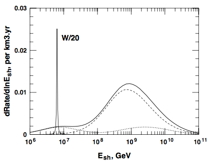
cannot occur in vacuum because it cannot simultaneously conserve energy and momentum. (Puzzle: why is this true? Answer below.) However, this process is allowed in the presence of a heavy nucleus that can absorb the additional momentum, as shown in the comic at the top of this post.

Muon  conversion experiments exploit this by forming muonic atoms in the 1state and waiting for the muon to convert into an electron which can then be detected. The upside is that all electrons from conversion have a fixed energy because they all come from the same initial state: 1s muonic aluminum at rest in the lab frame. This is in contrast with more common muon decay modes which involve two neutrinos and an electron; because this is a multibody final state, there is a smooth distribution of electron energies. This feature allows physicists to distinguish between the \mu \to e conversion versus the more frequent muon decay \mu \to e \nu_\mu \bar \nu_e in orbit or muon capture by the nucleus (similar to electron capture).

The Standard Model prediction for this rate is miniscule—it’s weighted by powers of the neutrino to the W boson mass ratio  (Puzzle: how does one see this? Answer below.). In fact, the current experimental bound on muon conversion comes from the Sindrum II experiment  looking at muonic gold which constrains the relative rate of muon conversion to muon capture by the gold nucleus to be less than 7 \times 10^{-13}
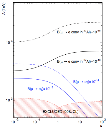
. This, in turn, constrains models of new physics that predict some level of charged lepton flavor violation—that is, processes that change the flavor of a charged lepton, say going from muons to electrons.

The plot on the right shows the energy scales that are indirectly probed by upcoming muonic aluminum experiments: the Mu2e experiment at Fermilab and the COMET experiment at J-PARC. The blue lines show bounds from another rare muon decay: muons decaying into an electron and photon. The black solid lines show the reach for muon conversion in muonic aluminum. The dashed lines correspond to different experimental sensitivities (capture rates for conversion, branching ratios for decay with a photon). Note that the energy scales probed can reach 1-10 PeV—that’s 1000-10,000 TeV—much higher than the energy scales direclty probed by the LHC! In this way, flavor experiments and high energy experiments are complimentary searches for new physics.

These “next generation” muon conversion experiments are currently under construction and promise to push the intensity frontier in conjunction with the LHC’s energy frontier.


Solutions to exercises:

  1. Why do pions decay into muons and not electrons? [Note: this requires some background in undergraduate-level particle physics.] One might expect that if a charged pion can decay into a muon and a neutrino, then it should also go into an electron and a neutrino. In fact, the latter should dominate since there’s much more phase space. However, the matrix element requires a virtual W boson exchange and thus depends on an [axial] vector current. The only vector available from the pion system is its 4-momentum. By momentum conservation this is $p_\pi = p_\mu + p_\nu$. The lepton momenta then contract with Dirac matrices on the leptonic current to give a dominant piece proportional to the lepton mass. Thus the amplitude for charged pion decay into a muon is much larger than the amplitude for decay into an electron.
  2. Why can’t a muon decay into an electron in vacuum? The process \mu \to e cannot simultaneously conserve energy and momentum. This is simplest to see in the reference frame where the muon is at rest. Momentum conservation requires the electron to also be at rest. However, a particle has rest energy equal to its mass, but now there’s now way a muon at rest can pass on all of its energy to an electron at rest.
  3. Why is muon conversion in the Standard Model suppressed by the ration of the neutrino to W masses? This can be seen by drawing the Feynman diagram (fig below from 1401.6077). Flavor violation in the Standard Model requires a W boson. Because the W is much heavier than the muon, this must be virtual and appear only as an internal leg. Further, W‘s couple charged leptons to neutrinos, so there must also be a virtual neutrino. The evaluation of this diagram into an amplitude gives factors of the neutrino mass in the numerator (required for the fermion chirality flip) and the W mass in the denominator. For some details, see this post.
    Screen Shot 2015-03-05 at 4.08.58 PM

Further Reading:

  • 1205.2671: Fundamental Physics at the Intensity Frontier (section 3.2.2)
  • 1401.6077: Snowmass 2013 Report, Intensity Frontier chapter


An update from AMS-02, the particle detector in space

Last Thursday, Nobel Laureate Sam Ting presented the latest results (CERN press release) from the Alpha Magnetic Spectrometer (AMS-02) experiment, a particle detector attached to the International Space Station—think “ATLAS/CMS in space.” Instead of beams of protons, the AMS detector examines cosmic rays in search of signatures of new physics such as the products of dark matter annihilation in our galaxy.

from http://ams.nasa.gov/images_AMS_On-Orbit.html
Image of AMS-02 on the space station, from NASA.

In fact, this is just the latest chapter in an ongoing mystery involving the energy spectrum of cosmic positrons. Recall that positrons are the antimatter versions of electrons with identical properties except having opposite charge. They’re produced from known astrophysical processes when high-energy cosmic rays (mostly protons) crash into interstellar gas—in this case they’re known as `secondaries’ because they’re a product of the `primary’ cosmic rays.

The dynamics of charged particles in the galaxy are difficult to simulate due to the presence of intense and complicated magnetic fields. However, the diffusion models generically predict that the positron fraction—the number of positrons divided by the total number of positrons and electrons—decreases with energy. (This ratio of fluxes is a nice quantity because some astrophysical uncertainties cancel.)

This prediction, however, is in stark contrast with the observed positron fraction from recent satellite experiments:

AMS-02, from http://physics.aps.org/articles/v6/40
Observed positron fraction from recent experiments compared to expected astrophysical background (gray) from APS viewpoint article based on the 2013 AMS-02 results (data) and the analysis in 1002.1910 (background).

The rising fraction had been hinted in balloon-based experiments for several decades, but the satellite experiments have been able to demonstrate this behavior conclusively because they can access higher energies. In their first set of results last year (shown above), AMS gave the most precise measurements of the positron fraction as far as 350 GeV. Yesterday’s announcement extended these results to 500 GeV and added the following observations:

First they claim that they have measured the maximum of the positron fraction to be 275 GeV. This is close to the edge of the data they’re releasing, but the plot of the positron fraction slope is slightly more convincing:

From Phys. Rev. Lett. 113, 121101
Lower: the latest positron fraction data from AMS-02 against a phenomenological model. Upper: slope of the lower curve. From Phys. Rev. Lett. 113, 121101. [Non-paywall summary.]
The observation of a maximum in what was otherwise a fairly featureless rising curve is key for interpretations of the excess, as we discuss below. A second observation is a bit more curious: while neither the electron nor the positron spectra follow a simple power law, \Phi_{e^\pm} \sim E^{-\delta}
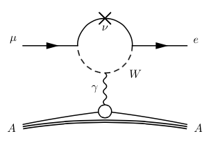
, the total electron or positron flux does follow such a power law over a range of energies.

...
Total electron/positron flux weighted by the cubed energy and the fit to a simple power law. From the AMS press summary.

This is a little harder to interpret since the flux form electrons also, in principle, includes different sources of background. Note that this plot reaches higher energies than the positron fraction—part of the reason for this is that it is more difficult to distinguish between electrons and positrons at high energies. This is because the identification depends on how the particle bends in the AMS magnetic field and higher energy particles bend less. This, incidentally, is also why the FERMI data has much larger error bars in the first plot above—FERMI doesn’t have its own magnetic field and must rely on that of the Earth for charge discrimination.

So what should one make of the latest results?

The most optimistic hope is that this is a signal of dark matter, and at this point this is more of a ‘wish’ than a deduction. Independently of AMS, we know is that dark matter exists in a halo that surrounds our galaxy. The simplest dark matter models also assume that when two dark matter particles find each other in this halo, they can annihilate into Standard Model particle–anti-particle pairs, such as electrons and positrons—the latter potentially yielding the rising positron fraction signal seen by AMS.

From a particle physics perspective, this would be the most exciting possibility. The ‘smoking gun’ signature of such a scenario would be a steep drop in the positron fraction at the mass of the dark matter particle. This is because the annihilation occurs at low velocities so that the energy of the annihilation products is set by the dark matter mass. This is why the observation of a maximum in the positron fraction is interesting: the dark matter interpretation of this excess hinges on how steeply the fraction drops off.

There are, however, reasons to be skeptical.

  • One attractive feature of dark matter annihilations is thermal freeze out: the observation that the annihilation rate determines how much dark matter exists today after being in thermal equilibrium in the early universe. The AMS excess is suggestive of heavy (~TeV scale) dark matter with an annihilation rate three orders of magnitude larger than the rate required for thermal freeze out.
  • A study of the types of spectra one expects from dark matter annihilation shows fits that are somewhat in conflict with the combined observations of the positron fraction, total electron/positron flux, and the anti-proton flux (see 0809.2409). The anti-proton flux, in particular, does not have any known excess that would otherwise be predicted by dark matter annihilation into quarks.

There are ways around these issues, such as invoking mechanisms to enhance the present day annihilation rate, perhaps with the annihilation only creating leptons and not quarks. However, these are additional bells and whistles that model-builders must impose on the dark matter sector. It is also important to consider alternate explanations of the Pamela/FERMI/AMS positron fraction excess due to astrophysical phenomena. There are at least two very plausible candidates:

  1. Pulsars are neutron stars that are known to emit “primary” electron/positron pairs. A nearby pulsar may be responsible for the observed rising positron fraction. See 1304.1791 for a recent discussion.
  2. Alternately, supernova remnants may also generate a “secondary” spectrum of positrons from acceleration along shock waves (0909.4060, 0903.2794, 1402.0855).

Both of these scenarios are plausible and should temper the optimism that the rising positron fraction represents a measurement of dark matter. One useful handle to disfavor the astrophysical interpretations is to note that they would be anisotropic (not constant over all directions) whereas the dark matter signal would be isotropic. See 1405.4884 for a recent discussion. At the moment, the AMS measurements do not measure any anisotropy but are not yet sensitive enough to rule out astrophysical interpretations.

Finally, let us also point out an alternate approach to understand the positron fraction. The reason why it’s so difficult to study cosmic rays is that the complex magnetic fields in the galaxy are intractable to measure and, hence, make the trajectory of charged particles hopeless to trace backwards to their sources. Instead, the authors of 0907.1686 and 1305.1324 take an alternate approach: while we can’t determine the cosmic ray origins, we can look at the behavior of heavier cosmic ray particles and compare them to the positrons. This is because, as mentioned above, the bending of a charged particle in a magnetic field is determined by its mass and charge—quantities that are known for the various cosmic ray particles. Based on this, the authors are able to predict an upper bound for the positron fraction when one assumes that the positrons are secondaries (e.g in the case of supernovae  remnant acceleration):

from  arXiv:1305.1324 , see Resonaances for an update
Upper bound on secondary positron fraction from 1305.1324. See Resonaances for an updated plot with last week’s data.

We see that the AMS-02 spectrum is just under the authors’ upper bound, and that the reported downturn is consistent with (even predicted from) the upper-bound. The authors’ analysis then suggests a non-dark matter explanation for the positron excess. See this post from Resonaances for a discussion of this point and an updated version of the above plot from the authors.

With that in mind, there are at least three things to look forward to in the future from AMS:

  1. A corresponding upturn in the anti-proton flux is predicted in many types of dark matter annihilation models for the rising positron fraction. Thus far AMS-02 has not released anti-proton data due to the lower numbers of anti-protons.
  2. Further sensitivity to the (an)isotropy of the excess is a critical test of the dark matter interpretation.
  3. The shape of the drop-off with energy is also critical: a gradual drop-off is unlikely to come from dark matter whereas a steep drop off is considered to be a smoking gun for dark matter.

Only time will tell; though Ting suggested that new results would be presented at the upcoming AMS meeting at CERN in 2 months.


Further reading:

This post was edited by Christine Muccianti.