Article: Search for TeV-scale gravity signatures in high-mass final states with leptons and jets with the ATLAS detector at sqrt(s)=13 TeV Authors: The ATLAS Collaboration Reference: arXiv:1606.02265 [hep-ex]
What would gravity look like if we lived in a 6-dimensional space-time? Models of TeV-scale gravity theorize that the fundamental scale of gravity, MD, is much lower than what’s measured here in our normal, 4-dimensional space-time. If true, this could explain the large difference between the scale of electroweak interactions (order of 100 GeV) and gravity (order of 1016 GeV), an important open question in particle physics. There are several theoretical models to describe these extra dimensions, and they all predict interesting new signatures in the form of non-perturbative gravitational states. One of the coolest examples of such a state is microscopic black holes. Conveniently, this particular signature could be produced and measured at the LHC!
Sounds cool, but how do you actually look for microscopic black holes with a proton-proton collider? Because we don’t have a full theory of quantum gravity (yet), ATLAS researchers made predictions for the production cross-sections of these black holes using semi-classical approximations that are valid when the black hole mass is above MD. This production cross-section is also expected to dramatically larger when the energy scale of the interactions (pp collisions) surpasses MD. We can’t directly detect black holes with ATLAS, but many of the decay channels of these black holes include leptons in the final state, which IS something that can be measured at ATLAS! This particular ATLAS search looked for final states with at least 3 high transverse momentum (pt) jets, at least one of which must be a leptonic (electron or muon) jet (the others can be hadronic or leptonic). The sum of the transverse momenta, is used as a discriminating variable since the signal is expected to appear only at high pt.
This search used the full 3.2 fb-1 of 13 TeV data collected by ATLAS in 2015 to search for this signal above relevant Standard Model backgrounds (Z+jets, W+jets, and ttbar, all of which produce similar jet final states). The results are shown in Figure 1 (electron and muon channels are presented separately). The various backgrounds are shown in various colored histograms, the data in black points, and two microscopic black hole models in green and blue lines. There is a slight excess in the 3 TeV region in the electron channel, which corresponds to a p-value of only 1% when tested against the background only hypothesis. Unfortunately, this isn’t enough evidence to indicate new physics yet, but it’s an exciting result nonetheless! This analysis was also used to improve exclusion limits on individual extra-dimensional gravity models, as shown in Figure 2. All limits were much stronger than those set in Run 1.
Figure 1: momentum distributions in the electron (a) and muon (b) channels
Figure 2: Exclusion limits in the Mth, MD plane for models with various numbers of extra dimensions
So: no evidence of microscopic black holes or extra-dimensional gravity at the LHC yet, but there is a promising excess and Run 2 has only just begun. Since publication, ATLAS has collected another 10 fb-1 of sqrt(13) TeV data that has yet to be analyzed. These results could also be used to constrain other Beyond the Standard Model searches at the TeV scale that have similar high pt leptonic jet final states, which would give us more information about what can and can’t exist outside of the Standard Model. There is certainly more to be learned from this search!
Article: Particle Physics Models for the 17 MeV Anomaly in Beryllium Nuclear Decays Authors: J.L. Feng, B. Fornal, I. Galon, S. Gardner, J. Smolinsky, T. M. P. Tait, F. Tanedo Reference:arXiv:1608.03591 (Submitted to Phys. Rev. D)
See also this Latin American Webinar on Physics recorded talk.
Also featuring the results from:
— Gulyás et al., “A pair spectrometer for measuring multipolarities of energetic nuclear transitions” (description of detector; 1504.00489; NIM)
— Krasznahorkay et al., “Observation of Anomalous Internal Pair Creation in 8Be: A Possible Indication of a Light, Neutral Boson” (experimental result; 1504.01527; PRL version; note PRL version differs from arXiv)
— Feng et al., “Protophobic Fifth-Force Interpretation of the Observed Anomaly in 8Be Nuclear Transitions” (phenomenology; 1604.07411; PRL)
Editor’s note: the author is a co-author of the paper being highlighted.
Recently there’s some press (see links below) regarding early hints of a new particle observed in a nuclear physics experiment. In this bite, we’ll summarize the result that has raised the eyebrows of some physicists, and the hackles of others.
A crash course on nuclear physics
Nuclei are bound states of protons and neutrons. They can have excited states analogous to the excited states of at lowoms, which are bound states of nuclei and electrons. The particular nucleus of interest is beryllium-8, which has four neutrons and four protons, which you may know from the triple alpha process. There are three nuclear states to be aware of: the ground state, the 18.15 MeV excited state, and the 17.64 MeV excited state.
Beryllium-8 excited nuclear states. The 18.15 MeV state (red) exhibits an anomaly. Both the 18.15 MeV and 17.64 states decay to the ground through a magnetic, p-wave transition. Image adapted from Savage et al. (1987).
Most of the time the excited states fall apart into a lithium-7 nucleus and a proton. But sometimes, these excited states decay into the beryllium-8 ground state by emitting a photon (γ-ray). Even more rarely, these states can decay to the ground state by emitting an electron–positron pair from a virtual photon: this is called internal pair creation and it is these events that exhibit an anomaly.
The beryllium-8 anomaly
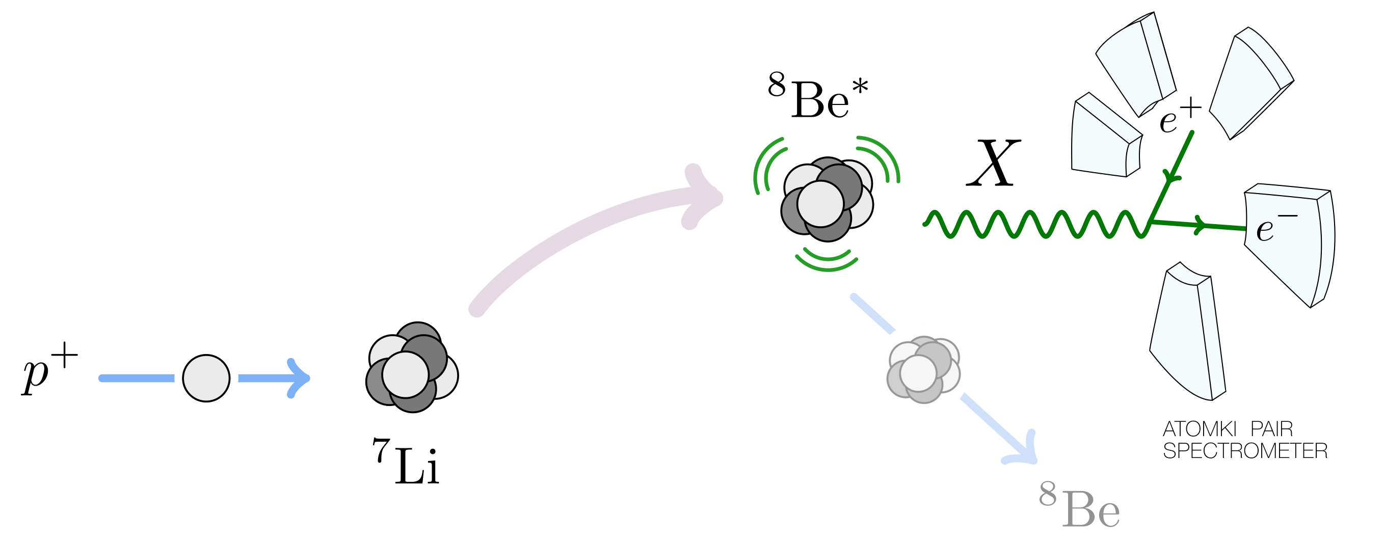
Physicists at the Atomki nuclear physics institute in Hungary were studying the nuclear decays of excited beryllium-8 nuclei. The team, led by Attila J. Krasznahorkay, produced beryllium excited states by bombarding a lithium-7 nucleus with protons.
Beryllium-8 excited states are prepare by bombarding lithium-7 with protons.
The proton beam is tuned to very specific energies so that one can ‘tickle’ specific beryllium excited states. When the protons have around 1.03 MeV of kinetic energy, they excite lithium into the 18.15 MeV beryllium state. This has two important features:
Picking the proton energy allows one to only produce a specific excited state so one doesn’t have to worry about contamination from decays of other excited states.
Because the 18.15 MeV beryllium nucleus is produced at resonance, one has a very high yield of these excited states. This is very good when looking for very rare decay processes like internal pair creation.
What one expects is that most of the electron–positron pairs have small opening angle with a smoothly decreasing number as with larger opening angles.
Expected distribution of opening angles for ordinary internal pair creation events. Each line corresponds to nuclear transition that is electric (E) or magenetic (M) with a given orbital quantum number, l. The beryllium transitionsthat we’re interested in are mostly M1. Adapted from Gulyás et al. (1504.00489).
Instead, the Atomki team found an excess of events with large electron–positron opening angle. In fact, even more intriguing: the excess occurs around a particular opening angle (140 degrees) and forms a bump.
Number of events (dN/dθ) for different electron–positron opening angles and plotted for different excitation energies (Ep). For Ep=1.10 MeV, there is a pronounced bump at 140 degrees which does not appear to be explainable from the ordinary internal pair conversion. This may be suggestive of a new particle. Adapted from Krasznahorkay et al., PRL 116, 042501.
Here’s why a bump is particularly interesting:
The distribution of ordinary internal pair creation events is smoothly decreasing and so this is very unlikely to produce a bump.
Bumps can be signs of new particles: if there is a new, light particle that can facilitate the decay, one would expect a bump at an opening angle that depends on the new particle mass.
Schematically, the new particle interpretation looks like this:
Schematic of the Atomki experiment and new particle (X) interpretation of the anomalous events. In summary: protons of a specific energy bombard stationary lithium-7 nuclei and excite them to the 18.15 MeV beryllium-8 state. These decay into the beryllium-8 ground state. Some of these decays are mediated by the new X particle, which then decays in to electron–positron pairs of a certain opening angle that are detected in the Atomki pair spectrometer detector. Image from 1608.03591.
As an exercise for those with a background in special relativity, one can use the relation to prove the result:
This relates the mass of the proposed new particle, X, to the opening angle θ and the energies E of the electron and positron. The opening angle bump would then be interpreted as a new particle with mass of roughly 17 MeV. To match the observed number of anomalous events, the rate at which the excited beryllium decays via the X boson must be 6×10⁻⁶ times the rate at which it goes into a γ-ray.
The anomaly has a significance of 6.8σ. This means that it’s highly unlikely to be a statistical fluctuation, as the 750 GeV diphoton bump appears to have been. Indeed, the conservative bet would be some not-understood systematic effect, akin to the 130 GeV Fermi γ-ray line.
The beryllium that cried wolf?
Some physicists are concerned that beryllium may be the ‘boy that cried wolf,’ and point to papers by the late Fokke de Boer as early as 1996 and all the way to 2001. de Boer made strong claims about evidence for a new 10 MeV particle in the internal pair creation decays of the 17.64 MeV beryllium-8 excited state. These claims didn’t pan out, and in fact the instrumentation paper by the Atomki experiment rules out that original anomaly.
The proposed evidence for “de Boeron” is shown below:
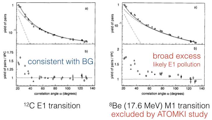
The de Boer claim for a 10 MeV new particle. Left: distribution of opening angles for internal pair creation events in an E1 transition of carbon-12. This transition has similar energy splitting to the beryllium-8 17.64 MeV transition and shows good agreement with the expectations; as shown by the flat “signal – background” on the bottom panel. Right: the same analysis for the M1 internal pair creation events from the 17.64 MeV beryllium-8 states. The “signal – background” now shows a broad excess across all opening angles. Adapted from de Boer et al. PLB 368, 235 (1996).
When the Atomki group studied the same 17.64 MeV transition, they found that a key background component—subdominant E1 decays from nearby excited states—dramatically improved the fit and were not included in the original de Boer analysis. This is the last nail in the coffin for the proposed 10 MeV “de Boeron.”
However, the Atomki group also highlight how their new anomaly in the 18.15 MeV state behaves differently. Unlike the broad excess in the de Boer result, the new excess is concentrated in a bump. There is no known way in which additional internal pair creation backgrounds can contribute to add a bump in the opening angle distribution; as noted above: all of these distributions are smoothly falling.
The Atomki group goes on to suggest that the new particle appears to fit the bill for a dark photon, a reasonably well-motivated copy of the ordinary photon that differs in its overall strength and having a non-zero (17 MeV?) mass.
Theory part 1: Not a dark photon
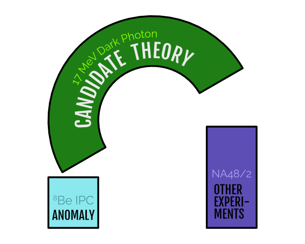
With the Atomki result was published and peer reviewed in Physics Review Letters, the game was afoot for theorists to understand how it would fit into a theoretical framework like the dark photon. A group from UC Irvine, University of Kentucky, and UC Riverside found that actually, dark photons have a hard time fitting the anomaly simultaneously with other experimental constraints. In the visual language of this recent ParticleBite, the situation was this:
It turns out that the minimal model of a dark photon cannot simultaneously explain the Atomki beryllium-8 anomaly without running afoul of other experimental constraints. Image adapted from this ParticleBite.
The main reason for this is that a dark photon with mass and interaction strength to fit the beryllium anomaly would necessarily have been seen by the NA48/2 experiment. This experiment looks for dark photons in the decay of neutral pions (π0). These pions typically decay into two photons, but if there’s a 17 MeV dark photon around, some fraction of those decays would go into dark-photon — ordinary-photon pairs. The non-observation of these unique decays rules out the dark photon interpretation.
The theorists then decided to “break” the dark photon theory in order to try to make it fit. They generalized the types of interactions that a new photon-like particle, X, could have, allowing protons, for example, to have completely different charges than electrons rather than having exactly opposite charges. Doing this does gross violence to the theoretical consistency of a theory—but they goal was just to see what a new particle interpretation would have to look like. They found that if a new photon-like particle talked to neutrons but not protons—that is, the new force were protophobic—then a theory might hold together.
Schematic description of how model-builders “hacked” the dark photon theory to fit both the beryllium anomaly while being consistent with other experiments. This hack isn’t pretty—and indeed, comes at the cost of potentially invalidating the mathematical consistency of the theory—but the exercise demonstrates the target for how to a complete theory might have to behave. Image adapted from this ParticleBite.
Theory appendix: pion-phobia is protophobia
Editor’s note: what follows is for readers with some physics background interested in a technical detail; others may skip this section.
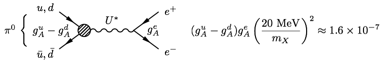
How does a new particle that is allergic to protons avoid the neutral pion decay bounds from NA48/2? Pions decay into pairs of photons through the well-known triangle-diagrams of the axial anomaly. The decay into photon–dark-photon pairs proceed through similar diagrams. The goal is then to make sure that these diagrams cancel.
A cute way to look at this is to assume that at low energies, the relevant particles running in the loop aren’t quarks, but rather nucleons (protons and neutrons). In fact, since only the proton can talk to the photon, one only needs to consider proton loops. Thus if the new photon-like particle, X, doesn’t talk to protons, then there’s no diagram for the pion to decay into γX. This would be great if the story weren’t completely wrong.
Avoiding NA48/2 bounds requires that the new particle, X, is pion-phobic. It turns out that this is equivalent to X being protophobic. The correct way to see this is on the left, making sure that the contribution of up-quark loops cancels the contribution from down-quark loops. A slick (but naively completely wrong) calculation is on the right, arguing that effectively only protons run in the loop.
The correct way of seeing this is to treat the pion as a quantum superposition of an up–anti-up and down–anti-down bound state, and then make sure that the X charges are such that the contributions of the two states cancel. The resulting charges turn out to be protophobic.
The fact that the “proton-in-the-loop” picture gives the correct charges, however, is no coincidence. Indeed, this was precisely how Jack Steinberger calculated the correct pion decay rate. The key here is whether one treats the quarks/nucleons linearly or non-linearly in chiral perturbation theory. The relation to the Wess-Zumino-Witten term—which is what really encodes the low-energy interaction—is carefully explained in chapter 6a.2 of Georgi’s revised Weak Interactions.
Theory part 2: Not a spin-0 particle
The above considerations focus on a new particle with the same spin and parity as a photon (spin-1, parity odd). Another result of the UCI study was a systematic exploration of other possibilities. They found that the beryllium anomaly could not be consistent with spin-0 particles. For a parity-odd, spin-0 particle, one cannot simultaneously conserve angular momentum and parity in the decay of the excited beryllium-8 state. (Parity violating effects are negligible at these energies.)
Parity and angular momentum conservation prohibit a “dark Higgs” (parity even scalar) from mediating the anomaly.
For a parity-odd pseudoscalar, the bounds on axion-like particles at 20 MeV suffocate any reasonable coupling. Measured in terms of the pseudoscalar–photon–photon coupling (which has dimensions of inverse GeV), this interaction is ruled out down to the inverse Planck scale.
Bounds on axion-like particles exclude a 20 MeV pseudoscalar with couplings to photons stronger than the inverse Planck scale. Adapted from 1205.2671 and 1512.03069.
Additional possibilities include:
Dark Z bosons, cousins of the dark photon with spin-1 but indeterminate parity. This is very constrained by atomic parity violation.
Axial vectors, spin-1 bosons with positive parity. These remain a theoretical possibility, though their unknown nuclear matrix elements make it difficult to write a predictive model. (See section II.D of 1608.03591.)
Theory part 3: Nuclear input
The plot thickens when once also includes results from nuclear theory. Recent results from Saori Pastore, Bob Wiringa, and collaborators point out a very important fact: the 18.15 MeV beryllium-8 state that exhibits the anomaly and the 17.64 MeV state which does not are actually closely related.
Recall (e.g. from the first figure at the top) that both the 18.15 MeV and 17.64 MeV states are both spin-1 and parity-even. They differ in mass and in one other key aspect: the 17.64 MeV state carries isospin charge, while the 18.15 MeV state and ground state do not.
Isospin is the nuclear symmetry that relates protons to neutrons and is tied to electroweak symmetry in the full Standard Model. At nuclear energies, isospin charge is approximately conserved. This brings us to the following puzzle:
If the new particle has mass around 17 MeV, why do we see its effects in the 18.15 MeV state but not the 17.64 MeV state?
Naively, if the new particle emitted, X, carries no isospin charge, then isospin conservation prohibits the decay of the 17.64 MeV state through emission of an X boson. However, the Pastore et al. result tells us that actually, the isospin-neutral and isospin-charged states mix quantum mechanically so that the observed 18.15 and 17.64 MeV states are mixtures of iso-neutral and iso-charged states. In fact, this mixing is actually rather large, with mixing angle of around 10 degrees!
The result of this is that one cannot invoke isospin conservation to explain the non-observation of an anomaly in the 17.64 MeV state. In fact, the only way to avoid this is to assume that the mass of the X particle is on the heavier side of the experimentally allowed range. The rate for X emission goes like the 3-momentum cubed (see section II.E of 1608.03591), so a small increase in the mass can suppresses the rate of X emission by the lighter state by a lot.
The UCI collaboration of theorists went further and extended the Pastore et al. analysis to include a phenomenological parameterization of explicit isospin violation. Independent of the Atomki anomaly, they found that including isospin violation improved the fit for the 18.15 MeV and 17.64 MeV electromagnetic decay widths within the Pastore et al. formalism. The results of including all of the isospin effects end up changing the particle physics story of the Atomki anomaly significantly:
The rate of X emission (colored contours) as a function of the X particle’s couplings to protons (horizontal axis) versus neutrons (vertical axis). The best fit for a 16.7 MeV new particle is the dashed line in the teal region. The vertical band is the region allowed by the NA48/2 experiment. Solid lines show the dark photon and protophobic limits. Left: the case for perfect (unrealistic) isospin. Right: the case when isospin mixing and explicit violation are included. Observe that incorporating realistic isospin happens to have only a modest effect in the protophobic region. Figure from 1608.03591.
The results of the nuclear analysis are thus that:
An interpretation of the Atomki anomaly in terms of a new particle tends to push for a slightly heavier X mass than the reported best fit. (Remark: the Atomki paper does not do a combined fit for the mass and coupling nor does it report the difficult-to-quantify systematic errors associated with the fit. This information is important for understanding the extent to which the X mass can be pushed to be heavier.)
The effects of isospin mixing and violation are important to include; especially as one drifts away from the purely protophobic limit.
Theory part 4: towards a complete theory
The theoretical structure presented above gives a framework to do phenomenology: fitting the observed anomaly to a particle physics model and then comparing that model to other experiments. This, however, doesn’t guarantee that a nice—or even self-consistent—theory exists that can stretch over the scaffolding.
Indeed, a few challenges appear:
The isospin mixing discussed above means the X mass must be pushed to the heavier values allowed by the Atomki observation.
The “protophobic” limit is not obviously anomaly-free: simply asserting that known particles have arbitrary charges does not generically produce a mathematically self-consistent theory.
Atomic parity violation constraints require that the X couple in the same way to left-handed and right-handed matter. The left-handed coupling implies that X must also talk to neutrinos: these open up new experimental constraints.
The Irvine/Kentucky/Riverside collaboration first note the need for a careful experimental analysis of the actual mass ranges allowed by the Atomki observation, treating the new particle mass and coupling as simultaneously free parameters in the fit.
Next, they observe that protophobic couplings can be relatively natural. Indeed: the Standard Model Z boson is approximately protophobic at low energies—a fact well known to those hunting for dark matter with direct detection experiments. For exotic new physics, one can engineer protophobia through a phenomenon called kinetic mixing where two force particles mix into one another. A tuned admixture of electric charge and baryon number, (Q-B), is protophobic.
Baryon number, however, is an anomalous global symmetry—this means that one has to work hard to make a baryon-boson that mixes with the photon (see 1304.0576 and 1409.8165 for examples). Another alternative is if the photon kinetically mixes with not baryon number, but the anomaly-free combination of “baryon-minus-lepton number,” Q-(B-L). This then forces one to apply additional model-building modules to deal with the neutrino interactions that come along with this scenario.
In the language of the ‘model building blocks’ above, result of this process looks schematically like this:
A complete theory is completely mathematically self-consistent and satisfies existing constraints. The additional bells and whistles required for consistency make additional predictions for experimental searches. Pieces of the theory can sometimes be used to address other anomalies.
The theory collaboration presented examples of the two cases, and point out how the additional ‘bells and whistles’ required may tie to additional experimental handles to test these hypotheses. These are simple existence proofs for how complete models may be constructed.
What’s next?
We have delved rather deeply into the theoretical considerations of the Atomki anomaly. The analysis revealed some unexpected features with the types of new particles that could explain the anomaly (dark photon-like, but not exactly a dark photon), the role of nuclear effects (isospin mixing and breaking), and the kinds of features a complete theory needs to have to fit everything (be careful with anomalies and neutrinos). The single most important next step, however, is and has always been experimental verification of the result.
While the Atomki experiment continues to run with an upgraded detector, what’s really exciting is that a swath of experiments that are either ongoing or in construction will be able to probe the exact interactions required by the new particle interpretation of the anomaly. This means that the result can be independently verified or excluded within a few years. A selection of upcoming experiments is highlighted in section IX of 1608.03591:
Other experiments that can probe the new particle interpretation of the Atomki anomaly. The horizontal axis is the new particle mass, the vertical axis is its coupling to electrons (normalized to the electric charge). The dark blue band is the target region for the Atomki anomaly. Figure from 1608.03591; assuming 100% branching ratio to electrons.
We highlight one particularly interesting search: recently a joint team of theorists and experimentalists at MIT proposed a way for the LHCb experiment to search for dark photon-like particles with masses and interaction strengths that were previously unexplored. The proposal makes use of the LHCb’s ability to pinpoint the production position of charged particle pairs and the copious amounts of D mesons produced at Run 3 of the LHC. As seen in the figure above, the LHCb reach with this search thoroughly covers the Atomki anomaly region.
Implications
So where we stand is this:
There is an unexpected result in a nuclear experiment that may be interpreted as a sign for new physics.
The next steps in this story are independent experimental cross-checks; the threshold for a ‘discovery’ is if another experiment can verify these results.
Meanwhile, a theoretical framework for understanding the results in terms of a new particle has been built and is ready-and-waiting. Some of the results of this analysis are important for faithful interpretation of the experimental results.
What if it’s nothing?
This is the conservative take—and indeed, we may well find that in a few years, the possibility that Atomki was observing a new particle will be completely dead. Or perhaps a source of systematic error will be identified and the bump will go away. That’s part of doing science.
Meanwhile, there are some important take-aways in this scenario. First is the reminder that the search for light, weakly coupled particles is an important frontier in particle physics. Second, for this particular anomaly, there are some neat take aways such as a demonstration of how effective field theory can be applied to nuclear physics (see e.g. chapter 3.1.2 of the new book by Petrov and Blechman) and how tweaking our models of new particles can avoid troublesome experimental bounds. Finally, it’s a nice example of how particle physics and nuclear physics are not-too-distant cousins and how progress can be made in particle–nuclear collaborations—one of the Irvine group authors (Susan Gardner) is a bona fide nuclear theorist who was on sabbatical from the University of Kentucky.
What if it’s real?
This is a big “what if.” On the other hand, a 6.8σ effect is not a statistical fluctuation and there is no known nuclear physics to produce a new-particle-like bump given the analysis presented by the Atomki experimentalists.
The threshold for “real” is independent verification. If other experiments can confirm the anomaly, then this could be a huge step in our quest to go beyond the Standard Model. While this type of particle is unlikely to help with the Hierarchy problem of the Higgs mass, it could be a sign for other kinds of new physics. One example is the grand unification of the electroweak and strong forces; some of the ways in which these forces unify imply the existence of an additional force particle that may be light and may even have the types of couplings suggested by the anomaly.
Could it be related to other anomalies?
The Atomki anomaly isn’t the first particle physics curiosity to show up at the MeV scale. While none of these other anomalies are necessarily related to the type of particle required for the Atomki result (they may not even be compatible!), it is helpful to remember that the MeV scale may still have surprises in store for us.
The KTeV anomaly: The rate at which neutral pions decay into electron–positron pairs appears to be off from the expectations based on chiral perturbation theory. In 0712.0007, a group of theorists found that this discrepancy could be fit to a new particle with axial couplings. If one fixes the mass of the proposed particle to be 20 MeV, the resulting couplings happen to be in the same ballpark as those required for the Atomki anomaly. The important caveat here is that parameters for an axial vector to fit the Atomki anomaly are unknown, and mixed vector–axial states are severely constrained by atomic parity violation.
The KTeV anomaly interpreted as a new particle, U. From 0712.0007.
The anomalous magnetic moment of the muon and the cosmic lithium problem: much of the progress in the field of light, weakly coupled forces comes from Maxim Pospelov. The anomalous magnetic moment of the muon, (g-2)μ, has a long-standing discrepancy from the Standard Model (see e.g. this blog post). While this may come from an error in the very, very intricate calculation and the subtle ways in which experimental data feed into it, Pospelov (and also Fayet) noted that the shift may come from a light (in the 10s of MeV range!), weakly coupled new particle like a dark photon. Similarly, Pospelov and collaborators showed that a new light particle in the 1-20 MeV range may help explain another longstanding mystery: the surprising lack of lithium in the universe (APS Physics synopsis).
The Proton Radius Problem: the charge radius of the proton appears to be smaller than expected when measured using the Lamb shift of muonic hydrogen versus electron scattering experiments. See this ParticleBite summary, and this recent review. Some attempts to explain this discrepancy have involved MeV-scale new particles, though the endeavor is difficult. There’s been some renewed popular interest after a new result using deuterium confirmed the discrepancy. However, there was a report that a result at the proton radius problem conference in Trento suggests that the 2S-4P determination of the Rydberg constant may solve the puzzle (though discrepant with other Rydberg measurements). [Those slides do not appear to be public.]
Could it be related to dark matter?
A lot of recent progress in dark matter has revolved around the possibility that in addition to dark matter, there may be additional light particles that mediate interactions between dark matter and the Standard Model. If these particles are light enough, they can change the way that we expect to find dark matter in sometimes surprising ways. One interesting avenue is called self-interacting dark matter and is based on the observation that these light force carriers can deform the dark matter distribution in galaxies in ways that seem to fit astronomical observations. A 20 MeV dark photon-like particle even fits the profile of what’s required by the self-interacting dark matter paradigm, though it is very difficult to make such a particle consistent with both the Atomki anomaly and the constraints from direct detection.
Should I be excited?
Given all of the caveats listed above, some feel that it is too early to be in “drop everything, this is new physics” mode. Others may take this as a hint that’s worth exploring further—as has been done for many anomalies in the recent past. For researchers, it is prudent to be cautious, and it is paramount to be careful; but so long as one does both, then being excited about a new possibility is part what makes our job fun.
For the general public, the tentative hopes of new physics that pop up—whether it’s the Atomki anomaly, or the 750 GeV diphoton bump, a GeV bump from the galactic center, γ-ray lines at 3.5 keV and 130 GeV, or penguins at LHCb—these are the signs that we’re making use of all of the data available to search for new physics. Sometimes these hopes fizzle away, often they leave behind useful lessons about physics and directions forward. Maybe one of these days an anomaly will stick and show us the way forward.
Further Reading
Here are some of the popular-level press on the Atomki result. See the references at the top of this ParticleBite for references to the primary literature.
Article: Probing Quarkonium Production Mechanisms with Jet Substructure Authors: Matthew Baumgart, Adam Leibovich, Thomas Mehen, and Ira Rothstein Reference: arXiv:1406.2295 [hep-ph]
“Tag…you’re it!” is a popular game to play with jets these days at particle accelerators like the LHC. These collimated sprays of radiation are common in various types of high-energy collisions and can present a nasty challenge to both theorists and experimentalists (for more on the basic ideas and importance of jet physics, see my July bite on the subject). The process of tagging a jet generally means identifying the type of particle that initiated the jet. Since jets provide a significant contribution to backgrounds at high energy colliders, identifying where they come from can make doing things like discovering new particles much easier. While identifying backgrounds to new physics is important, in this bite I want to focus on how theorists are now using jets to study the production of hadrons in a unique way.
Over the years, a host of theoretical tools have been developed for making the study of jets tractable. The key steps of “reconstructing” jets are:
Choose a jet algorithm (i.e. basically pick a metric that decides which particles it thinks are “clustered”),
Identify potential jet axes (i.e. the centers of the jets),
Decide which particles are in/out of the jets based on your jet algorithm.
Figure 1: A basic 3-jet event where one of the reconstructed jets is found to have been initiated by a b quark. The process of finding such jets is called “tagging.”
Deciphering the particle content of a jet can often help to uncover what particle initiated the jet. While this is often enough for many analyses, one can ask the next obvious question: how are the momenta of the particles within the jet distributed? In other words, what does the inner geometry of the jet look like?
There are a number of observables that one can look at to study a jet’s geometry. These are generally referred to as jet substructure observables. Two basic examples are:
Jet-shape: This takes a jet of radius R and then identifies a sub-jet within it of radius r. By measuring the energy fraction contained within sub-jets of variable radius r, one can study where the majority of the jet’s energy/momentum is concentrated.
Jet mass: By measuring the invariant mass of all of the particles in a jet (while simultaneously considering the jet’s energy and radius) one can gain insight into how focused a jet is.
Figure 2: A basic way to produce quarkonium via the fragmentation of a gluon. The interactions highlighted in blue are calculated using standard perturbative QCD. The green zone is where things get tricky and non-perturbative models that are extracted from data must often be used.
One way in which phenomenologists are utilizing jet substructure technology is in the study of hadron production. In arXiv:1406.2295, Baumgart et. al. introduced a way to connect the world of jet physics with the world of quarkonia. These bound states of charm-anti-charm or bottom-anti-bottom quarks are the source of two things: great buzz words for impressing your friends and several outstanding problems within the standard model. While we’ve been studying quarkonia such the and the for a half-century, there are still a bunch of very basic questions we have about how they are produced (more on this topic in future bites).
This paper offers a fresh approach to studying the various ways in which quarkonia are produced at the LHC by focusing on how they are produced within jets. The wealth of available jet physics technology then provides a new family of interesting observables. The authors first describe the various mechanisms by which quarkonia are produced. In the formalism of Non-relativistic (NR) QCD, the for example, is most frequently produced at the LHC (see Fig. 2) when a high energy gluon splits into a pair in one of several possible angular momentum and color quantum states. This pair then ultimately undergoes non-perturbative (i.e. we can’t really calculate them using standard techniques in quantum field theory) effects and becomes a color-singlet final state particle (as any reasonably minded particle should do). While this model makes some sense, we have no idea how often quarkonia are produced via each mechanism.
Figure 3: This plot from arXiv:1406.2295 shows how the probability that a gluon or quark fragments into a jet with a specific energy E that a contains a with a fraction of the original quark/gluon’s momentum varies for different mechanisms. The spectroscopic notation should be familiar from basic quantum mechanics. It gives the angular momentum and color quantum numbers of the pair that eventually becomes quarkonium. Notice that for different values of z and E, the different mechanisms behave differently. Thus this observable (i.e. that mouth full of a probability distribution I described) is said to have discriminating power between the different channels by which a is typically formed.
This paper introduces a theoretical formalism that looks at the following question: what is the probability that a parton (quark/gluon) hadronizes into a jet with a certain substructure and that contains a specific hadron with some fraction of the original partons energy? The authors show that the answer to this question is correlated with the answer to the question: How often are quarkonia produced via the different intermediate angular-momentum/color states of NRQCD? In other words, they show that studying how the geometry of the jets that contain quarkonia may lead to answers to decades old questions about how quarkonia are produced!
There are several other efforts to study hadron production through the lens of jet physics that have also done preliminary comparisons with ATLAS/CMS data (one such study will be the subject of my next bite). These studies look at the production of more general classes of hadrons and numbers of jets in events and see promising results when compared with 7 TeV data from ATLAS and CMS.
The moral of this story is that jets are now being viewed less as a source of troublesome backgrounds to new physics and more as a laboratory for studying long-standing questions about the underlying nature of hadronization. Jet physics offers innovative ways to look at old problems, offering a host of new and exciting observables to study at the LHC and other experiments.
Further Reading
The November Revolution: https://www.slac.stanford.edu/history/pubs/gilmannov.pdf. This transcript of a talk provides some nice background on, amongst other things, the momentous discovery of the in 1974 what is often referred to the November Revolution.
An Introduction to the NRQCD Factorization Approach to Heavy Quarkoniumhttps://cds.cern.ch/record/319642/files/9702225.pdf. As good as it gets when it comes to outlines of the basics of this tried-and-true effective theory. This article will definitely take some familiarity with QFT but provides a great outline of the basics of the NRQCD Lagrangian, fields, decays etc.
One thing that makes physics, and especially particle physics, is unique in the sciences is the split between theory and experiment. The role of experimentalists is clear: they build and conduct experiments, take data and analyze it using mathematical, statistical, and numerical techniques to separate signal from background. In short, they seem to do all of the real science!
So what is it that theorists do, besides sipping espresso and scribbling on chalk boards? In this post we describe one type of theoretical work called model building. This usually falls under the umbrella of phenomenology, which in physics refers to making connections between mathematically defined theories (or models) of nature and actual experimental observations of nature.
One common scenario is that one experiment observes something unusual: an anomaly. Two things immediately happen:
Other experiments find ways to cross-check to see if they can confirm the anomaly.
Theorists start figure out the broader implications if the anomaly is real.
#1 is the key step in the scientific method, but in this post we’ll illuminate what #2 actually entails. The scenario looks a little like this:
An unusual experimental result (anomaly) is observed. One thing we would like to know is whether it is consistent with other experimental observations, but these other observations may not be simply related to the anomaly.
Theorists, who have spent plenty of time mulling over the open questions in physics, are ready to apply their favorite models of new physics to see if they fit. These are the models that they know lead to elegant mathematical results, like grand unification or a solution to the Hierarchy problem. Sometimes theorists are more utilitarian, and start with “do it all” Swiss army knife theories called effective theories (or simplified models) and see if they can explain the anomaly in the context of existing constraints.
Here’s what usually happens:
Usually the nicest models of new physics don’t fit! In the explicit example, the minimal supersymmetric Standard Model doesn’t include a good candidate to explain the 750 GeV diphoton bump.
Indeed, usually one needs to get creative and modify the nice-and-elegant theory to make sure it can explain the anomaly while avoiding other experimental constraints. This makes the theory a little less elegant, but sometimes nature isn’t elegant.
Candidate theory extended with a module (in this case, an additional particle). This additional model is “bolted on” to the theory to make it fit the experimental observations.
Now we’re feeling pretty good about ourselves. It can take quite a bit of work to hack the well-motivated original theory in a way that both explains the anomaly and avoids all other known experimental observations. A good theory can do a couple of other things:
It points the way to future experiments that can test it.
It can use the additional structure to explain other anomalies.
The picture for #2 is as follows:
A good hack to a theory can explain multiple anomalies. Sometimes that makes the hack a little more cumbersome. Physicists often develop their own sense of ‘taste’ for when a module is elegant enough.
Even at this stage, there can be a lot of really neat physics to be learned. Model-builders can develop a reputation for particularly clever, minimal, or inspired modules. If a module is really successful, then people will start to think about it as part of a pre-packaged deal:
A really successful hack may eventually be thought of as it’s own variant of the original theory.
Model-smithing is a craft that blends together a lot of the fun of understanding how physics works—which bits of common wisdom can be bent or broken to accommodate an unexpected experimental result? Is it possible to find a simpler theory that can explain more observations? Are the observations pointing to an even deeper guiding principle?
Of course—we should also say that sometimes, while theorists are having fun developing their favorite models, other experimentalists have gone on to refute the original anomaly.
Sometimes anomalies go away and the models built to explain them don’t hold together.
But here’s the mark of a really, really good model: even if the anomaly goes away and the particular model falls out of favor, a good model will have taught other physicists something really neat about what can be done within the a given theoretical framework. Physicists get a feel for the kinds of modules that are out in the market (like an app store) and they develop a library of tricks to attack future anomalies. And if one is really fortunate, these insights can point the way to even bigger connections between physical principles.
I cannot help but end this post without one of my favorite physics jokes, courtesy of T. Tait:
A theorist and an experimentalist are having coffee. The theorist is really excited, she tells the experimentalist, “I’ve got it—it’s a model that’s elegant, explains everything, and it’s completely predictive.”
The experimentalist listens to her colleague’s idea and realizes how to test those predictions. She writes several grant applications, hires a team of postdocs and graduate students, trains them, and builds the new experiment. After years of design, labor, and testing, the machine is ready to take data. They run for several months, and the experimentalist pores over the results.
The experimentalist knocks on the theorist’s door the next day and says, “I’m sorry—the experiment doesn’t find what you were predicting. The theory is dead.”
The theorist frowns a bit: “What a shame. Did you know I spent three whole weeks of my life writing that paper?”
Article: Detection of the pairwise kinematic Sunyaev-Zel’dovich effect with BOSS DR11 and the Atacama Cosmology Telescope Authors: F. De Bernardis, S. Aiola, E. M. Vavagiakis, M. D. Niemack, N. Battaglia, and the ACT Collaboration Reference:arXiv:1607.02139
Editor’s note: this post is written by one of the students involved in the published result.
Like X-rays shining through your body can inform you about your health, the cosmic microwave background (CMB) shining through galaxy clusters can tell us about the universe we live in. When light from the CMB is distorted by the high energy electrons present in galaxy clusters, it’s called the Sunyaev-Zel’dovich effect. A new 4.1σ measurement of the kinematic Sunyaev-Zel’dovich (kSZ) signal has been made from the most recent Atacama Cosmology Telescope (ACT) cosmic microwave background (CMB) maps and galaxy data from the Baryon Oscillation Spectroscopic Survey (BOSS). With steps forward like this one, the kinematic Sunyaev-Zel’dovich signal could become a probe of cosmology, astrophysics and particle physics alike.
The Kinematic Sunyaev-Zel’dovich Effect
It rolls right off the tongue, but what exactly is the kinematic Sunyaev-Zel’dovich signal? Galaxy clusters distort the cosmic microwave background before it reaches Earth, so we can learn about these clusters by looking at these CMB distortions. In our X-ray metaphor, the map of the CMB is the image of the X-ray of your arm, and the galaxy clusters are the bones. Galaxy clusters are the largest gravitationally bound structures we can observe, so they serve as important tools to learn more about our universe. In its essence, the Sunyaev-Zel’dovich effect is inverse-Compton scattering of cosmic microwave background photons off of the gas in these galaxy clusters, whereby the photons gain a “kick” in energy by interacting with the high energy electrons present in the clusters.
The Sunyaev-Zel’dovich effect can be divided up into two categories: thermal and kinematic. The thermal Sunyaev-Zel’dovich (tSZ) effect is the spectral distortion of the cosmic microwave background in a characteristic manner due to the photons gaining, on average, energy from the hot (~107 – 108 K) gas of the galaxy clusters. The kinematic (or kinetic) Sunyaev-Zel’dovich (kSZ) effect is a second-order effect—about a factor of 10 smaller than the tSZ effect—that is caused by the motion of galaxy clusters with respect to the cosmic microwave background rest frame. If the CMB photons pass through galaxy clusters that are moving, they are Doppler shifted due to the cluster’s peculiar velocity (the velocity that cannot be explained by Hubble’s law, which states that objects recede from us at a speed proportional to their distance). The kinematic Sunyaev-Zel’dovich effect is the only known way to directly measure the peculiar velocities of objects at cosmological distances, and is thus a valuable source of information for cosmology. It allows us to probe megaparsec and gigaparsec scales – that’s around 30,000 times the diameter of the Milky Way!
A schematic of the Sunyaev-Zel’dovich effect resulting in higher energy (or blue shifted) photons of the cosmic microwave background (CMB) when viewed through the hot gas present in galaxy clusters. Source: UChicago Astronomy.
Measuring the kSZ Effect
To make the measurement of the kinematic Sunyaev-Zel’dovich signal, the Atacama Cosmology Telescope (ACT) collaboration used a combination of cosmic microwave background maps from two years of observations by ACT. The CMB map used for the analysis overlapped with ~68000 galaxy sources from the Large Scale Structure (LSS) DR11 catalog of the Baryon Oscillation Spectroscopic Survey (BOSS). The catalog lists the coordinate positions of galaxies along with some of their properties. The most luminous of these galaxies were assumed to be located at the centers of galaxy clusters, so temperature signals from the CMB map were taken at the coordinates of these galaxy sources in order to extract the Sunyaev-Zel’dovich signal.
While the smallness of the kSZ signal with respect to the tSZ signal and the noise level in current CMB maps poses an analysis challenge, there exist several approaches to extracting the kSZ signal. To make their measurement, the ACT collaboration employed a pairwise statistic. “Pairwise” refers to the momentum between pairs of galaxy clusters, and “statistic” indicates that a large sample is used to rule out the influence of unwanted effects.
Here’s the approach: nearby galaxy clusters move towards each other on average, due to gravity. We can’t easily measure the three-dimensional momentum of clusters, but the average pairwise momentum can be estimated by using the line of sight component of the momentum, along with other information such as redshift and angular separations between clusters. The line of sight momentum is directly proportional to the measured kSZ signal: the microwave temperature fluctuation which is measured from the CMB map. We want to know if we’re measuring the kSZ signal when we look in the direction of galaxy clusters in the CMB map. Using the observed CMB temperature to find the line of sight momenta of galaxy clusters, we can estimate the mean pairwise momentum as a function of cluster separation distance, and check to see if we find that nearby galaxies are indeed falling towards each other. If so, we know that we’re observing the kSZ effect in action in the CMB map.
For the measurement quoted in their paper, the ACT collaboration finds the average pairwise momentum as a function of galaxy cluster separation, and explores a variety of error determinations and sources of systematic error. The most conservative errors based on simulations give signal-to-noise estimates that vary between 3.6 and 4.1.
The mean pairwise momentum estimator and best fit model for a selection of 20000 objects from the DR11 Large Scale Structure catalog, plotted as a function of comoving separation. The dashed line is the linear model, and the solid line is the model prediction including nonlinear redshift space corrections. The best fit provides a 4.1σ evidence of the kSZ signal in the ACTPol-ACT CMB map. Source: arXiv:1607.02139.
The ACT and BOSS results are an improvement on the 2012 ACT detection, and are comparable with results from the South Pole Telescope (SPT) collaboration that use galaxies from the Dark Energy Survey. The ACT and BOSS measurement represents a step forward towards improved extraction of kSZ signals from CMB maps. Future surveys such as Advanced ACTPol, SPT-3G, the Simons Observatory, and next-generation CMB experiments will be able to apply the methods discussed here to improved CMB maps in order to achieve strong detections of the kSZ effect. With new data that will enable better measurements of galaxy cluster peculiar velocities, the pairwise kSZ signal will become a powerful probe of our universe in the years to come.
Implications and Future Experiments
One interesting consequence for particle physics will be more stringent constraints on the sum of the neutrino masses from the pairwise kinematic Sunyaev-Zel’dovich effect. Upper bounds on the neutrino mass sum from cosmological measurements of large scale structure and the CMB have the potential to determine the neutrino mass hierarchy, one of the next major unknowns of the Standard Model to be resolved, if the mass hierarchy is indeed a “normal hierarchy” with ν3 being the heaviest mass state. If the upper bound of the neutrino mass sum is measured to be less than 0.1 eV, the inverted hierarchy scenario would be ruled out, due to there being a lower limit on the mass sum of ~0.095 eV for an inverted hierarchy and ~0.056 eV for a normal hierarchy.
Forecasts for kSZ measurements in combination with input from Planck predict possible constraints on the neutrino mass sum with a precision of 0.29 eV, 0.22 eV and 0.096 eV for Stage II (ACTPol + BOSS), Stage III (Advanced ACTPol + BOSS) and Stage IV (next generation CMB experiment + DESI) surveys respectively, with the possibility of much improved constraints with optimal conditions. As cosmic microwave background maps are improved and Sunyaev-Zel’dovich analysis methods are developed, we have a lot to look forward to.
Article: Forecasting the Socio-Economic Impact of the Large Hadron Collider: a Cost-Benefit Analysis to 2025 and Beyond Authors: Massimo Florio, Stefano Forte, Emanuela Sirtori Reference:arXiv:1603.00886v1 [physics.soc-ph]
Imagine this. You’re at a party talking to a non-physicist about your research.
If this scenario already has you cringing, imagine you’re actually feeling pretty encouraged this time. Your everyday analogy for the Higgs mechanism landed flawlessly and you’re even getting some interested questions in return. Right when you’re feeling like Neil DeGrasse Tyson himself, your flow grinds to a halt and you have to stammer an awkward answer to the question every particle physicist has nightmares about.
“Why are we spending so much money to discover these fundamental particles? Don’t they seem sort of… useless?”
Well, fair question. While us physicists simply get by with a passion for the field, a team of Italian economists actually did the legwork on this one. And they came up with a really encouraging answer.
The paper being summarized here performed a cost-benefit analysis of the LHC from 1993 to 2025, in order to estimate its eventual impact on the world at large. Not only does that include benefit to future scientific endeavors, but to industry and even the general public as well. To do this, they called upon some classic non-physics notions, so let’s start with a quick economics primer.
A cost benefit analysis (CBA) is a common thing to do before launching a large-scale investment project. The LHC collaboration is a particularly tough thing to analyze; it is massive, international, complicated, and has a life span of several decades.
In general, basic research is notoriously difficult to justify to funding agencies, since there are no immediate applications. (A similar problem is encountered with environmental CBAs, so there are some overlapping ideas between the two.) Something that taxpayers fund without getting any direct use of the end product is referred to as a non-use value.
When trying to predict the future gets fuzzy, economists define something called a quasi option value. For the LHC, this includes aspects of timing and resource allocation (for example, what potential quality-of-life benefits come from discovering supersymmetry, and how bad would it have been if we pushed these off another 100 years?)
One can also make a general umbrella term for the benefit of pure knowledge, called an existence value. This involves a sort of social optimization; basically what taxpayers are willing to pay to get more knowledge.
The actual equation used to represent the different costs and benefits at play here is below.
Let’s break this down by terms.
PVCu is the sum of operating costs and capital associated with getting the project off the ground and continuing its operation.
PVBu is the economic value of the benefits. Here is where we have to break down even further, into who is benefitting and what they get out of it:
Scientists, obviously. They get to publish new research and keep having jobs. Same goes for students and post-docs.
Technological industry. Not only do they get wrapped up in the supply chain of building these machines, but basic research can quickly turn into very profitable new ideas for private companies.
Everyone else. Because it’s fun to tour the facilities or go to public lectures. Plus CERN even has an Instagram now.
Just to give you an idea of how much overlap there really is between all these sources of benefit, Figure 1 shows the monetary amount of goods procured from industry for the LHC. Figure 2 shows the number of ROOT software downloads, which, if you are at all familiar with ROOT, may surprise you (yes, it really is very useful outside of HEP!)
Figure 1: Amount of money (thousands of Euros) spent on industry for the LHC. pCp is past procurement, tHp1 is the total high tech procurement, and tHp2 is the high tech procurement for orders > 50 kCHF.Figure 2: Number of ROOT software downloads over time.
The rightmost term encompasses the non-use value, which is the difference between the sum of the quasi-option value QOV0 and existence value EXV0. If it sounded hard to measure a quasi-option value, it really is. In fact, the authors of this paper simply set it to 0, as a worst case value.
The other values come from in-depth interviews of over 1500 people, including all different types of physicists and industry representatives, as well as previous research papers. This data is then funneled into a computable matrix model, with a cell for each cost/benefit variable, for each year in the LHC lifetime. One can then create a conditional probability distribution function for the NPV value using Monte Carlo simulations to deal with the stochastic variables.
The end PDF is shown in Figure 2, with an expected NPV of 2.9 billion Euro! This also shows a expected benefit/cost ratio of 1.2; a project is generally considered justifiable if this ratio is greater than 1. If this all seems terribly exciting (it is), it never hurts to contact your Congressman and tell them just how much you love physics. It may not seem like much, but it will help ensure that the scientific community continues to get projects on the level of the LHC, even during tough federal budget times.
Figure 3: Net present value PDF (left) and cumulative distribution (right).
Here’s hoping this article helped you avoid at least one common source of awkwardness at a party. Unfortunately we can’t help you field concerns about the LHC destroying the world. You’re on your own with that one.
Further Reading:
Another supercollider that didn’t get so lucky: The SSC story
Article: Search for resonant production of high mass photon pairs using 12.9/fb of proton-proton collisions at √s = 13 TeV and combined interpretation of searches at 8 and 13 TeV Authors: CMS Collaboration Reference:CERN Document Server (CMS-PAS-EXO-16-027, presented at ICHEP)
In the early morning hours of Friday, August 5th, the particle physics community let our a collective, exasperated sigh. What some knew, others feared, and everyone gossiped about was announced publicly at the 38th International Conference on High Energy Physics: the 750 GeV bump had vanished.
Had it endured, the now-defunct “diphoton bump” would have been the highlight of ICHEP, a biennial meeting of the high energy physics community currently being held in Chicago, Illinois. In light of this, the scheduling of the announcements for a parallel session in the middle of the conference – rather than a specially arranged plenary session – said anything that the rumors had not already: there would be no need for champagne or press releases.
While the exact statistical significance depends upon the width and spin of the resonance in question, meaning that the paper presents multiple p-value plots corresponding to different signal hypotheses, the following plot is a good representative.
Combined background-only p-values for a new scalar particle in the CMS diphoton data from both 2015 and 2016. The dip in blue near 750 GeV is the excess observed during 2015, and the flat red line indicates the result from the 2016 data: no excess. Had a new particle existed at 750 GeV, we would have expected to see a similar dip in the red curve.
We hoped that the 2016 LHC dataset would bring confirmation that the excess seen during 2015 was evidence of a new particle, but instead, the 2016 data has assured us that 2015 was merely a statistical fluctuation. When combining the data currently available from 8 TeV and 13 TeV, the excess at 750 GeV is reduced to <2σ local significance. The channel with the largest, which was 3.4σ local significance excess before the addition of 2016 data, has now been reduced to 1.9 sigma local significance, and other channels have seen analogous drops. As a result, CMS reports that “no significant excess” is observed over the Standard Model predictions.
The excess disappearing was clearly the less-desirable of the two possible outcomes, but is there a silver lining here? This CMS result puts the most stringent limits to date on the production of Randall-Sundrum (RS) gravitons, and the excitement generated by the diphoton bump sparked a flurry of activity within the theory community. A discovery would have been preferred to exclusion limits, and the papers published concerned a signal that has subsequently disappeared, but I would argue that both of these help our field move forward.
However, as we continue to push exclusion limits further across all manner of search for new physics, particle physicists become understandably antsy. Across all manner of searches for supersymmetry and exotica, the jump in energy from 8 to 13 TeV has allowed us to place more stringent exclusion limits. This is great news, but it is not the flurry of discoveries that some hoped the increase in energy during Run II would bring. It seems that there was no new physics ready to jump out and surprise us at the outset of Run II, so if we are to discover new physics at the LHC in the coming years, we will need to pick it out of the mountains of background. New physics may be lurking nearby, but if we want it, we will have to work harder to get it.
References and Further Reading
CERN Press, “Chicago sees floods of LHC data and new results at the ICHEP 2016 Conference” (link)
Alessandro Strumia, “Interpreting the 750 GeV digamma excess: a review” (arXiv:1605.09401)
Title: Estimating the GeV Emission of Millisecond Pulsars in Dwarf Spheroidal Galaxies Publication: arXiv: 1607.06390, submitted to ApJL
Howdy, particlebite enthusiasts! I’m blogging this week from ICHEP. Over the next week there will be a lot of exciting updates from the particle physics community… like what happened to that 750 GeV bump? are there any new bumps for us to be excited about? have we broken the standard model yet? But all these will come later in the week – today is registration. But in the mean time, there have been a lot of interesting papers circulating about disentangling dark matter from our favorite astrophysical background – pulsars.
The paper, which is the focus of this post, delves deeper into understanding potential gamma-ray emission found in dwarf spheroidal galaxies (dsphs) from pulsars. The density of millisecond pulsars (MSPs) is related to the density of stars in a cluster. In low-density stellar environments, such as dsphs, the abundance of MSPs is expected to be proportional to stellar mass (it’s much higher for globular cluster and the Galactic center). Remember, the advantage over dsphs in looking for a dark matter signal when compared with, for example, the Galactic center is that they have many fewer detectable gamma-ray emitting sources – like MSPs (see arXiv: 1503.02641 for a recent Fermi-LAT paper). However, as we get more and more sensitive, the probability of detecting gamma rays from astrophysical sources in dsphs goes up as well.
MSP gamma-ray luminosity function (0.1–100 GeV) normalized to the stellar mass of the Milky Way. The shaded gray band represents the 1σ statistical uncertainty on the broken power-law fit to these data and dashed gray lines represent the systematic uncertainty envelope.
This work estimates what the gamma-ray flux should be (known as the luminosity function) for MSPs found in dsphs. They assume that the number of MSPs is proportional to the stellar density and that the spectrum is similar to the 90 known MSPs in the Galactic disk (see the figure on the right). It fits the gamma-ray spectrum to a broken power law. We can then scale this result to the number of predicted MSPs in each dsph and distance of the dsph. This is then used as a prediction of the gamma-ray spectrum we would expect from MSPs coming from an individual dsph.
They found was that for the highest stellar mass dsphs (Fornax, Draco – usually the classical ones, for example), there is a modest MSP population. However, even for the largest classical dsph, Fornax, the predicted MSP flux > 500 MeV is~ 10−12 ph cm−2s−1 , which is about an order of magnitude below the typical flux upper limits obtained at high Galactic latitudes after six years of the LAT survey, ∼ 10−10 ph cm−2s−1 (see arXiv: 1503.02641 again). The predicted flux and sensitivity is shown below.
Expected flux versus J-factor (remember J-factor scales with distance). Blue points indicate the predicted MSP contribution in 30 Milky Way dsphs and dsph candidates. The gray shaded band represents the sensitivity for 6 years of the LAT data. The red curve represents a DM annihilation model that is consistent with both DM interpretations of the Galactic Center Excess and the characteristic spectral shape of MSPs.
So all in all, this is good news for dsphs as dark matter targets. Understanding the backgrounds is imperative for having confidence in an analysis if a signal is found, and this gives us more confidence that we understand one of the dominant backgrounds in the hunt for dark matter.


 to prove the result:


 and the
  for a half-century, there are still a bunch of very basic questions we have about how they are produced (more on this topic in future bites).
 for example, is most frequently produced at the LHC (see Fig. 2) when a high energy gluon splits into a
  pair in one of several possible angular momentum and color quantum states. This pair then ultimately undergoes non-perturbative (i.e. we can’t really calculate them using standard techniques in quantum field theory) effects and becomes a color-singlet final state particle (as any reasonably minded particle should do). While this model makes some sense, we have no idea how often quarkonia are produced via each mechanism.
 of the original quark/gluon’s momentum varies for different mechanisms. The spectroscopic notation should be familiar from basic quantum mechanics. It gives the angular momentum and color quantum numbers of the
  pair that eventually becomes quarkonium. Notice that for different values of z and E, the different mechanisms behave differently. Thus this observable (i.e. that mouth full of a probability distribution I described) is said to have discriminating power between the different channels by which a


