jets – ParticleBites

December 18, 2020December 18, 2020

Machine Learning The LHC ABC’s

Article Title: ABCDisCo: Automating the ABCD Method with Machine Learning

Authors: Gregor Kasieczka, Benjamin Nachman, Matthew D. Schwartz, David Shih

Reference: arxiv:2007.14400

When LHC experiments try to look for the signatures of new particles in their data they always apply a series of selection criteria to the recorded collisions. The selections pick out events that look similar to the sought after signal. Often they then compare the observed number of events passing these criteria to the number they would expect to be there from ‘background’ processes. If they see many more events in real data than the predicted background that is evidence of the sought after signal. Crucial to whole endeavor is being able to accurately estimate the number of events background processes would produce. Underestimate it and you may incorrectly claim evidence of a signal, overestimate it and you may miss the chance to find a highly sought after signal.

However it is not always so easy to estimate the expected number of background events. While LHC experiments do have high quality simulations of the Standard Model processes that produce these backgrounds they aren’t perfect. Particularly processes involving the strong force (aka Quantum Chromodynamics, QCD) are very difficult to simulate, and refining these simulations is an active area of research. Because of these deficiencies we don’t always trust background estimates based solely on these simulations, especially when applying very specific selection criteria.

Therefore experiments often employ ‘data-driven’ methods where they estimate the amount background events by using control regions in the data. One of the most widely used techniques is called the ABCD method.

An illustration of the ABCD method. The signal region, A, is defined as the region in which f and g are greater than some value. The amount of background in region A is estimated using regions B C and D which are dominated by background.

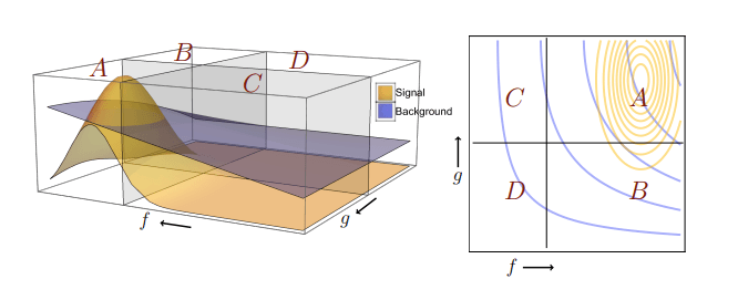
The ABCD method can applied if the selection of signal-like events involves two independent variables f and g. If one defines the ‘signal region’, A, (the part of the data in which we are looking for a signal) as having f and g each greater than some amount, then one can use the neighboring regions B, C, and D to estimate the amount of background in region A. If the number of signal events outside region A is small, the number of background events in region A can be estimated as N_A = N_B * (N_C/N_D).

In modern analyses often one of these selection requirements involves the score of a neural network trained to identify the sought after signal. Because neural networks are powerful learners one often has to be careful that they don’t accidentally learn about the other variable that will be used in the ABCD method, such as the mass of the signal particle. If two variables become correlated, a background estimate with the ABCD method will not be possible. This often means augmenting the neural network either during training or after the fact so that it is intentionally ‘de-correlated’ with respect to the other variable. While there are several known techniques to do this, it is still a tricky process and often good background estimates come with a trade off of reduced classification performance.

In this latest work the authors devise a way to have the neural networks help with the background estimate rather than hindering it. The idea is rather than training a single network to classify signal-like events, they simultaneously train two networks both trying to identify the signal. But during this training they use a groovy technique called ‘DisCo’ (short for Distance Correlation) to ensure that these two networks output is independent from each other. This forces the networks to learn to use independent information to identify the signal. This then allows these networks to be used in an ABCD background estimate quite easily.

The authors try out this new technique, dubbed ‘Double DisCo’, on several examples. They demonstrate they are able to have quality background estimates using the ABCD method while achieving great classification performance. They show that this method improves upon the previous state of the art technique of decorrelating a single network from a fixed variable like mass and using cuts on the mass and classifier to define the ABCD regions (called ‘Single Disco’ here).

Using the task of identifying jets containing boosted top quarks, they compare the classification performance (x-axis) and quality of the ABCD background estimate (y-axis) achievable with the new Double DisCo technique (yellow points) and previously state of the art Single DisCo (blue points). One can see the Double DisCo method is able to achieve higher background rejection with a similar or better amount of ABCD closure.

While there have been many papers over the last few years about applying neural networks to classification tasks in high energy physics, not many have thought about how to use them to improve background estimates as well. Because of their importance, background estimates are often the most time consuming part of a search for new physics. So this technique is both interesting and immediately practical to searches done with LHC data. Hopefully it will be put to use in the near future!

A shortcut to truth

Article title: “Automated detector simulation and reconstruction
parametrization using machine learning”

Authors: D. Benjamin, S.V. Chekanov, W. Hopkins, Y. Li, J.R. Love

Reference: https://arxiv.org/abs/2002.11516 (https://iopscience.iop.org/article/10.1088/1748-0221/15/05/P05025)

Demonstration of probability density function as the output of a neural network. (Source: paper)

The simulation of particle collisions at the LHC is a pharaonic task. The messy chromodynamics of protons must be modeled; the statistics of the collision products must reflect the Standard Model; each particle has to travel through the detectors and interact with all the elements in its path. Its presence will eventually be reduced to electronic measurements, which, after all, is all we know about it.

The work of the simulation ends somewhere here, and that of the reconstruction starts; namely to go from electronic signals to particles. Reconstruction is a process common to simulation and to the real world. Starting from the tangle of statistical and detector effects that the actual measurements include, the goal is to divine the properties of the initial collision products.

Now, researchers at the Argonne National Laboratory looked into going from the simulated particles as produced in the collisions (aka “truth objects”) directly to the reconstructed ones (aka “reco objects”): bypassing the steps of the detailed interaction with the detectors and of the reconstruction algorithm could make the studies that use simulations much more speedy and efficient.

Display of a collision event involving hadronic jets at ATLAS. Each colored block corresponds to interaction with a detector element. (Source: ATLAS experiment)

The team used a neural network which it trained on simulations of the full set. The goal was to have the network learn to produce the properties of the reco objects when given only the truth objects. The process succeeded in producing the transverse momenta of hadronic jets, and looks suitable for any kind of particle and for other kinematic quantities.

More specifically, the researchers began with two million simulated jet events, fully passed through the ATLAS experiment and the reconstruction algorithm. For each of them, the network took the kinematic properties of the truth jet as input and was trained to achieve the reconstructed transverse momentum.

The network was taught to perform multi-categorization: its output didn’t consist of a single node giving the momentum value, but of 400 nodes, each corresponding to a different range of values. The output of each node was the probability for that particular range. In other words, the result was a probability density function for the reconstructed momentum of a given jet.

The final step was to select the momentum randomly from this distribution. For half a million of test jets, all this resulted in good agreement with the actual reconstructed momenta, specifically within 5% for values above 20 GeV. In addition, it seems that the training was sensitive to the effects of quantities other than the target one (e.g. the effects of the position in the detector), as the neural network was able to pick up on the dependencies between the input variables. Also, hadronic jets are complicated animals, so it is expected that the method will work on other objects just as well.

Comparison of the reconstructed transverse momentum between the full simulation and reconstruction (“Delphes”) and the neural net output. (Source: paper)

All in all, this work showed the perspective for neural networks to imitate successfully the effects of the detector and the reconstruction. Simulations in large experiments typically take up loads of time and resources due to their size, intricacy and frequent need for updates in the hardware conditions. Such a shortcut, needing only small numbers of fully processed events, would speed up studies such as optimization of the reconstruction and detector upgrades.

More reading:

Argonne Lab press release: https://www.anl.gov/article/learning-more-about-particle-collisions-with-machine-learning

Intro to neural networks: https://physicsworld.com/a/neural-networks-explained/

November 19, 2019November 19, 2019

CMS catches the top quark running

CMS catches the top quark running

Article : “Running of the top quark mass from proton-proton collisions at √ s = 13 TeV“

Authors: The CMS Collaboration

Reference: https://arxiv.org/abs/1909.09193

When theorists were first developing quantum field theory in the 1940’s they quickly ran into a problem. Some of their calculations kept producing infinities which didn’t make physical sense. After scratching their heads for a while they eventually came up with a procedure known as renormalization to solve the problem. Renormalization neatly hid away the infinities that were plaguing their calculations by absorbing them into the constants (like masses and couplings) in the theory, but it also produced some surprising predictions. Renormalization said that all these ‘constants’ weren’t actually constant at all! The value of these ‘constants’ depended on the energy scale at which you probed the theory.

One of the most famous realizations of this phenomena is the ‘running’ of the strong coupling constant. The value of a coupling encodes the strength of a force. The strong nuclear force, responsible for holding protons and neutrons together, is actually so strong at low energies our normal techniques for calculation don’t work. But in 1973, Gross, Wilczek and Politzer realized that in quantum chromodynamics (QCD), the quantum field theory describing the strong force, renormalization would make the strong coupling constant ‘run’ smaller at high energies. This meant at higher energies one could use normal perturbative techniques to do calculations. This behavior of the strong force is called ‘asymptotic freedom’ and earned them a Nobel prize. Thanks to asymptotic freedom, it is actually much easier for us to understand what QCD predicts for high energy LHC collisions than for the properties of bound states like the proton.

Figure 1: The value of the strong coupling constant (α_s) is plotted as a function of the energy scale. Data from multiple experiments at different energies are compared to the prediction from QCD of how it should run. From [5]

Now for the first time, CMS has measured the running of a new fundamental parameter, the mass of the top quark. More than just being a cool thing to see, measuring how the top quark mass runs tests our understanding of QCD and can also be sensitive to physics beyond the Standard Model. The top quark is the heaviest fundamental particle we know about, and many think that it has a key role to play in solving some puzzles of the Standard Model. In order to measure the top quark mass at different energies, CMS used the fact that the rate of producing a top quark-antiquark pair depends on the mass of the top quark. So by measuring this rate at different energies they can extract the top quark mass at different scales.

Top quarks nearly always decay into W-bosons and b quarks. Like all quarks, the b quarks then create a large shower of particles before they reach the detector called a jet. The W-bosons can decay either into a lepton and a neutrino or two quarks. The CMS detector is very good at reconstructing leptons and jets, but neutrinos escape undetected. However one can infer the presence of neutrinos in an event because we know energy must be conserved in the collision, so if neutrinos are produced we will see ‘missing’ energy in the event. The CMS analyzers looked for top anti-top pairs where one W-boson decayed to an electron and a neutrino and the other decayed to a muon and a neutrino. By using information about the electron, muon, missing energy, and jets in an event, the kinematics of the top and anti-top pair can be reconstructed.

The measured running of the top quark mass is shown in Figure 2. The data agree with the predicted running from QCD at the level of 1.1 sigma, and the no-running hypothesis is excluded at above 95% confidence level. Rather than being limited by the amount of data, the main uncertainties in this result come from the theoretical understanding of the top quark production and decay, which the analyzers need to model very precisely in order to extract the top quark mass. So CMS will need some help from theorists if they want to improve this result in the future.

Figure 2: The ratio of the top quark mass compared to its mass at a reference scale (476 GeV) is plotted as a function of energy. The red line is the theoretical prediction of how the mass should run in QCD.

“The Strengths of Known Forces” https://profmattstrassler.com/articles-and-posts/particle-physics-basics/the-known-forces-of-nature/the-strength-of-the-known-forces/
“Renormalization Made Easy” http://math.ucr.edu/home/baez/renormalization.html
“Studying the Higgs via Top Quark Couplings” https://particlebites.com/?p=4718
“The QCD Running Coupling” https://arxiv.org/abs/1604.08082
CMS Measurement of QCD Running Coupling https://arxiv.org/abs/1609.05331

October 28, 2016February 27, 2017

What Happens When Energy Goes Missing?

Title: “Performance of algorithms that reconstruct missing transverse momentum in s = √8 TeV proton–proton collisions in the ATLAS detector”
Authors: ATLAS Collaboration

Reference: arXiv:1609.09324

Check out the public version of this post on the official ATLAS blog here!

The ATLAS experiment recently released a note detailing the nature and performance of algorithms designed to calculate what is perhaps the most difficult quantity in any LHC event: missing transverse energy. Missing energy is difficult because by its very nature, it is missing, thus making it unobservable in the detector. So where does this missing energy come from, and why do we even need it?

The LHC accelerate protons towards one another on the same axis, so they will collide head on. Therefore, the incoming partons have net momentum along the direction of the beamline, but no net momentum in the transverse direction (see Figure 1). MET is then defined as the negative vectorial sum (in the transverse plane) of all recorded particles. Any nonzero MET indicates a particle that escaped the detector. This escaping particle could be a regular Standard Model neutrino, or something much more exotic, such as the lightest supersymmetric particle or a dark matter candidate.

Figure 2 shows an event display where the calculated MET balances the visible objects in the detector. In this case, these visible objects are jets, but they could also be muons, photons, electrons, or taus. This constitutes the “hard term” in the MET calculation. Often there are also contributions of energy in the detector that are not associated to a particular physics object, but may still be necessary to get an accurate measurement of MET. This momenta is known as the “soft term”.

In the course of looking at all the energy in the detector for a given event, inevitably some pileup will sneak in. The pileup could be contributions from additional proton-proton collisions in the same bunch crossing, or from scattering of protons upstream of the interaction point. Either way, the MET reconstruction algorithms have to take this into account. Adding up energy from pileup could lead to more MET than was actually in the collision, which could mean the difference between an observation of dark matter and just another Standard Model event.

One of the ways to suppress pile up is to use a quantity called jet vertex fraction (JVF), which uses the additional information of tracks associated to jets. If the tracks do not point back to the initial hard scatter, they can be tagged as pileup and not included in the calculation. This is the idea behind the Track Soft Term (TST) algorithm. Another way to remove pileup is to estimate the average energy density in the detector due to pileup using event-by-event measurements, then subtracting this baseline energy. This is used in the Extrapolated Jet Area with Filter, or EJAF algorithm.

Once these algorithms are designed, they are tested in two different types of events. One of these is in W to lepton + neutrino decay signatures. These events should all have some amount of real missing energy from the neutrino, so they can easily reveal how well the reconstruction is working. The second group is Z boson to two lepton events. These events should not have any real missing energy (no neutrinos), so with these events, it is possible to see if and how the algorithm reconstructs fake missing energy. Fake MET often comes from miscalibration or mismeasurement of physics objects in the detector. Figures 3 and 4 show the calorimeter soft MET distributions in these two samples; here it is easy to see the shape difference between real and fake missing energy.

Figure 3: Distribution of the sum of missing energy in the calorimeter soft term shown in Z to μμ data and Monte Carlo events.

Figure 4: Distribution of the sum of missing energy in the calorimeter soft term shown in W to eν data and Monte Carlo events.

This note evaluates the performance of these algorithms in 8 TeV proton proton collision data collected in 2012. Perhaps the most important metric in MET reconstruction performance is the resolution, since this tells you how well you know your MET value. Intuitively, the resolution depends on detector resolution of the objects that went into the calculation, and because of pile up, it gets worse as the number of vertices gets larger. The resolution is technically defined as the RMS of the combined distribution of MET in the x and y directions, covering the full transverse plane of the detector. Figure 5 shows the resolution as a function of the number of vertices in Z to μμ data for several reconstruction algorithms. Here you can see that the TST algorithm has a very small dependence on the number of vertices, implying a good stability of the resolution with pileup.

Figure 5: Distribution of the sum of missing energy in the calorimeter soft term shown in W to eν data and Monte Carlo events.

Another important quantity to measure is the angular resolution, which is important in the reconstruction of kinematic variables such as the transverse mass of the W. It can be measured in W to μν simulation by comparing the direction of the MET, as reconstructed by the algorithm, to the direction of the true MET. The resolution is then defined as the RMS of the distribution of the phi difference between these two vectors. Figure 6 shows the angular resolution of the same five algorithms as a function of the true missing transverse energy. Note the feature between 40 and 60 GeV, where there is a transition region into events with high pT calibrated jets. Again, the TST algorithm has the best angular resolution for this topology across the entire range of true missing energy.

Figure 6: Resolution of ΔΦ(reco MET, true MET) for 0 jet W to μν Monte Carlo.

As the High Luminosity LHC looms larger and larger, the issue of MET reconstruction will become a hot topic in the ATLAS collaboration. In particular, the HLLHC will be a very high pile up environment, and many new pile up subtraction studies are underway. Additionally, there is no lack of exciting theories predicting new particles in Run 3 that are invisible to the detector. As long as these hypothetical invisible particles are being discussed, the MET teams will be working hard to catch them.

August 23, 2016February 19, 2017

Jets aren’t just a game of tag anymore

Article: Probing Quarkonium Production Mechanisms with Jet Substructure
Authors: Matthew Baumgart, Adam Leibovich, Thomas Mehen, and Ira Rothstein
Reference: arXiv:1406.2295 [hep-ph]

“Tag…you’re it!” is a popular game to play with jets these days at particle accelerators like the LHC. These collimated sprays of radiation are common in various types of high-energy collisions and can present a nasty challenge to both theorists and experimentalists (for more on the basic ideas and importance of jet physics, see my July bite on the subject). The process of tagging a jet generally means identifying the type of particle that initiated the jet. Since jets provide a significant contribution to backgrounds at high energy colliders, identifying where they come from can make doing things like discovering new particles much easier. While identifying backgrounds to new physics is important, in this bite I want to focus on how theorists are now using jets to study the production of hadrons in a unique way.

Over the years, a host of theoretical tools have been developed for making the study of jets tractable. The key steps of “reconstructing” jets are:

Choose a jet algorithm (i.e. basically pick a metric that decides which particles it thinks are “clustered”),
Identify potential jet axes (i.e. the centers of the jets),
Decide which particles are in/out of the jets based on your jet algorithm.

Figure 1: A basic 3-jet event where one of the reconstructed jets is found to have been initiated by a b quark. The process of finding such jets is called "tagging." — Figure 1: A basic 3-jet event where one of the reconstructed jets is found to have been initiated by a b quark. The process of finding such jets is called “tagging.”

Deciphering the particle content of a jet can often help to uncover what particle initiated the jet. While this is often enough for many analyses, one can ask the next obvious question: how are the momenta of the particles within the jet distributed? In other words, what does the inner geometry of the jet look like?

There are a number of observables that one can look at to study a jet’s geometry. These are generally referred to as jet substructure observables. Two basic examples are:

Jet-shape: This takes a jet of radius R and then identifies a sub-jet within it of radius r. By measuring the energy fraction contained within sub-jets of variable radius r, one can study where the majority of the jet’s energy/momentum is concentrated.
Jet mass: By measuring the invariant mass of all of the particles in a jet (while simultaneously considering the jet’s energy and radius) one can gain insight into how focused a jet is.

Figure 2: A basic way to produce quarkonium via the fragmentation of a gluon. The interactions highlighted in blue are calculated using standard perturbative QCD. The green zone is where things get tricky and non-perturbative models that are extracted from data must be used. — Figure 2: A basic way to produce quarkonium via the fragmentation of a gluon. The interactions highlighted in blue are calculated using standard perturbative QCD. The green zone is where things get tricky and non-perturbative models that are extracted from data must often be used.

One way in which phenomenologists are utilizing jet substructure technology is in the study of hadron production. In arXiv:1406.2295, Baumgart et. al. introduced a way to connect the world of jet physics with the world of quarkonia. These bound states of charm-anti-charm or bottom-anti-bottom quarks are the source of two things: great buzz words for impressing your friends and several outstanding problems within the standard model. While we’ve been studying quarkonia such the $J/\psi(c\bar{c})$ and the $\Upsilon(b\bar{b})$ for a half-century, there are still a bunch of very basic questions we have about how they are produced (more on this topic in future bites).

This paper offers a fresh approach to studying the various ways in which quarkonia are produced at the LHC by focusing on how they are produced within jets. The wealth of available jet physics technology then provides a new family of interesting observables. The authors first describe the various mechanisms by which quarkonia are produced. In the formalism of Non-relativistic (NR) QCD, the $J/\psi$ for example, is most frequently produced at the LHC (see Fig. 2) when a high energy gluon splits into a $c\bar{c}$ pair in one of several possible angular momentum and color quantum states. This pair then ultimately undergoes non-perturbative (i.e. we can’t really calculate them using standard techniques in quantum field theory) effects and becomes a color-singlet final state particle (as any reasonably minded particle should do). While this model makes some sense, we have no idea how often quarkonia are produced via each mechanism.

Figure 3: This plot from arXiv:1406.2295 shows how the probability that a gluon or quark fragments into a jet with a specific energy E that a contains a $latex J/\psi$ with a fraction $latex z$ of the original quark/gluon's momentum varies for different mechanisms. The spectroscopic notation should be familiar from basic quantum mechanics. It gives the angular momentum and color quantum numbers of the $latex q\bar{q}$ pair that eventually becomes quarkonium. Notice that for different values of z and E, the different mechanisms behave differently. — Figure 3: This plot from arXiv:1406.2295 shows how the probability that a gluon or quark fragments into a jet with a specific energy E that a contains a $J/\psi$ with a fraction $z$ of the original quark/gluon’s momentum varies for different mechanisms. The spectroscopic notation should be familiar from basic quantum mechanics. It gives the angular momentum and color quantum numbers of the $q\bar{q}$ pair that eventually becomes quarkonium. Notice that for different values of z and E, the different mechanisms behave differently. Thus this observable (i.e. that mouth full of a probability distribution I described) is said to have *discriminating power* between the different channels by which a $J/\psi$ is typically formed.

Figure 3: This plot from arXiv:1406.2295 shows how the probability that a gluon or quark fragments into a jet with a specific energy E that a contains a $J/\psi$ with a fraction $z$ of the original quark/gluon’s momentum varies for different mechanisms. The spectroscopic notation should be familiar from basic quantum mechanics. It gives the angular momentum and color quantum numbers of the $q\bar{q}$ pair that eventually becomes quarkonium. Notice that for different values of z and E, the different mechanisms behave differently. Thus this observable (i.e. that mouth full of a probability distribution I described) is said to have *discriminating power* between the different channels by which a $J/\psi$ is typically formed.

This paper introduces a theoretical formalism that looks at the following question: what is the probability that a parton (quark/gluon) hadronizes into a jet with a certain substructure and that contains a specific hadron with some fraction $z$ of the original partons energy? The authors show that the answer to this question is correlated with the answer to the question: How often are quarkonia produced via the different intermediate angular-momentum/color states of NRQCD? In other words, they show that studying how the geometry of the jets that contain quarkonia may lead to answers to decades old questions about how quarkonia are produced!

There are several other efforts to study hadron production through the lens of jet physics that have also done preliminary comparisons with ATLAS/CMS data (one such study will be the subject of my next bite). These studies look at the production of more general classes of hadrons and numbers of jets in events and see promising results when compared with 7 TeV data from ATLAS and CMS.

The moral of this story is that jets are now being viewed less as a source of troublesome backgrounds to new physics and more as a laboratory for studying long-standing questions about the underlying nature of hadronization. Jet physics offers innovative ways to look at old problems, offering a host of new and exciting observables to study at the LHC and other experiments.

Further Reading

The November Revolution: https://www.slac.stanford.edu/history/pubs/gilmannov.pdf. This transcript of a talk provides some nice background on, amongst other things, the momentous discovery of the $J/\psi$ in 1974 what is often referred to the November Revolution.
An Introduction to the NRQCD Factorization Approach to Heavy Quarkonium https://cds.cern.ch/record/319642/files/9702225.pdf. As good as it gets when it comes to outlines of the basics of this tried-and-true effective theory. This article will definitely take some familiarity with QFT but provides a great outline of the basics of the NRQCD Lagrangian, fields, decays etc.

July 26, 2016February 19, 2017

Jets: More than Riff, Tony, and a rumble

Review Bite: Jet Physics
(This is the first in a series of posts on jet physics by Reggie Bain.)

Ubiquitous in the LHC’s ultra-high energy collisions are collimated sprays of particles called jets. The study of jet physics is a rapidly growing field where experimentalists and theorists work together to unravel the complex geometry of the final state particles at LHC experiments. If you’re totally new to the idea of jets…this bite from July 18th, 2016 by Julia Gonski is a nice experimental introduction to the importance of jets. In this bite, we’ll look at the basic ideas of jet physics from a more theoretical perspective. Let’
s address a few basic questions:

What is a jet? Jets are highly collimated collections of particles that are frequently observed in detectors. In visualizations of collisions in the ATLAS detector, one can often identify jets by eye.

A nicely colored visualization of a multi-jet event in the ATLAS detector. Reason #172 that I’m not an experimentalist...actually sifting out useful information from the detector (or even making a graphic like this) is insanely hard. — A nicely colored visualization of a multi-jet event in the ATLAS detector. Reason #172 that I’m not an experimentalist…actually sifting out useful information from the detector (or even making a graphic like this) is insanely hard.

Jets are formed in the final state of a collision when a particle showers off radiation in such a way as to form a focused cone of particles. The most commonly studied jets are formed by quarks and gluons that fragment into hadrons like pions, kaons, and sometimes more exotic particles like the $latex J/Ψ, Υ, χ_c and many others. This process is often referred to as hadronization.

Why do jets exist? Jets are a fundamental prediction of Quantum Field Theories like Quantum Chromodynamics (QCD). One common process studied in field theory textbooks is electron–positron annihilation into a pair of quarks, e⁺e^– → q q. In order to calculate the
cross-section of this process, it turns out that one has to consider the possibility that additional gluons are produced along with the qq. Since no detector has infinite resolution, it’s always possible that there are gluons that go unobserved by your detector. This could be because they are incredibly soft (low energy) or because they travel almost exactly collinear to the q or q itself. In this region of momenta, the cross-section gets very large and the process favors the creation of this extra radiation. Since these gluons carry color/anti-color, they begin to hadronize and decay so as to become stable, colorless states. When the q, q have high momenta, the zoo of particles that are formed from the hadronization all have momenta that are clustered around the direction of the original q,q and form a cone shape in the detector…thus a jet is born! The details of exactly how hadronization works is where theory can get a little hazy. At the energy and distance scales where quarks/gluons start to hadronize, perturbation theory breaks down making many of our usual calculational tools useless. This, of course, makes the realm of hadronization—often referred to as parton fragmentation in the literature—a hot topic in QCD research.

How do we measure/study jets? Now comes the tricky part. As experimentalists will tell you, actually measuring jets can a messy business. By taking the signatures of the final state particles in an event (i.e. a collision), one can reconstruct a jet using a jet algorithm. One of the first concepts of such jet definitions was introduced by Geroge Sterman and Steven Weinberg in 1977. There they defined a jet using two parameters θ, E. These restricted the angle and energy of particles that are in or out of a jet. Today, we have a variety of jet algorithms that fall into two categories:

Cone Algorithms — These algorithms identify stable cones of a given angular size. These cones are defined in such a way that if one or two nearby particles are added to or removed from the jet cone, that it won’t drastically change the cone location and energy
Recombination Algorithms — These look pairwise at the 4-momenta of all particles in an event and combine them, according to a certain distance metric (there’s a different one for each algorithm), in such a way as to be left with distinct, well-separated jets.

Figure 2: From Cacciari and Salam’s original paper on the “Anti-kT” jet algorithm (See arXiv:0802.1189). The picture shows the application of 4 different jet algorithms: the kT, Cambridge/Aachen, Seedless-Infrared-Safe Cone, and anti-kT algorithms to a single set of final state particles in an event. You can see how each algorithm reconstructs a slightly different jet structure. These are among the most commonly used clustering algorithms on the market (the anti-kT being, at least in my experience, the most popular).

Why are jets important? On the frontier of high energy particle physics, CERN leads the world’s charge in the search for new physics. From deepening our understanding of the Higgs to observing never before seen particles, projects like ATLAS,

An illustration of an interesting type of jet substructure observable called “N-subjettiness” from the original paper by Jesse Thaler and Ken van Tilburg (see arXiv:1011.2268). N-subjettiness aims to study how momenta within a jet are distributed by dividing them up into n sub-jets. The diagram on the left shows an example of 2-subjettiness where a jet contains two sub-jets. The diagram on the right shows a jet with 0 sub-jets.

CMS, and LHCb promise to uncover interesting physics for years to come. As it turns out, a large amount of Standard Model background to these new physics discoveries comes in the form of jets. Understanding the origin and workings of these jets can thus help us in the search for physics beyond the Standard Model.

Additionally, there are a number of interesting questions that remain about the Standard Model itself. From studying the production of heavy hadron production/decay in pp and heavy-ion collisions to providing precision measurements of the strong coupling, jets physics has a wide range of applicability and relevance to Standard Model problems. In recent years, the physics of jet substructure, which studies the distributions of particle momenta within a jet, has also seen increased interest. By studying the geometry of jets, a number of clever observables have been developed that can help us understand what particles they come from and how they are formed. Jet substructure studies will be the subject of many future bites!

Going forward…With any luck, this should serve as a brief outline to the uninitiated on the basics of jet physics. In a world increasingly filled with bigger, faster, and stronger colliders, jets will continue to play a major role in particle phenomenology. In upcoming bites, I’ll discuss the wealth of new and exciting results coming from jet physics research. We’ll examine questions like:

How do theoretical physicists tackle problems in jet physics?
How does the process of hadronization/fragmentation of quarks and gluons really work?
Can jets be used to answer long outstanding problems in the Standard Model?

I’ll also bite about how physicists use theoretical smart bombs called “effective field theories” to approach these often nasty theoretical calculations. But more on that later…