Uncategorized – Page 4 – ParticleBites

March 1, 2021March 1, 2021

Maleficent dark matter: Part I

We might not have gotten here without dark matter. It was the gravitational pull of dark matter, which makes up most of the mass of galactic structures, that kept heavy elements — the raw material of Earth-like rocky planets — from flying away after the first round of supernovae at the advent of the stelliferous era. Without this invisible pull, all structures would have been much smaller than seen today, and stars much more rare.

Thus with knowledge of dark matter comes existential gratitude. But the microscopic identity of dark matter is one of the biggest scientific enigmas of our times, and what we don’t know could yet kill us. This two-part series is about the dangerous end of our ignorance, reviewing some inconvenient prospects sketched out in the dark matter literature. Reader discretion is advised.

[Note: The scenarios outlined here are based on theoretical speculations of dark matter’s identity. Such as they are, these are unlikely to occur, and even if they do, extremely unlikely within the lifetime of our species, let alone that of an individual. In other words, nobody’s sleep or actuarial tables need be disturbed.]

The dark matter wind could blow in mischief. Image source: Freese et al.

Carcinogenic dark matter

Maurice Goldhaber quipped that “you could feel it in your bones” that protons are cosmologically long-lived, as otherwise our bodies would have self-administered a lethal dose of ionizing radiation. (This observation sets a lower limit on the proton lifetime at a comforting $10^7$ times the age of the universe.) Could we laugh similarly about dark matter? The Earth is probably amid a wind of particle dark matter, a wind that could trigger fatal ionization in our cells if encountered too frequently. The good news is that if dark matter is made of weakly interacting massive particles (WIMPs), K. Freese and C. Savage report safety: “Though WIMP interactions are a source of radiation in the body, the annual exposure is negligible compared to that from other natural sources (including radon and cosmic rays), and the WIMP collisions are harmless to humans.“

The bad news is that the above statement assumes dark matter is distributed smoothly in the Galactic halo. There are interesting cosmologies in which dark matter collects in high-density “clumps” (a.k.a. “subhalos”, “mini-halos”, or “mini-clusters”). According to J. I. Collar, the Earth encountering these clumps every 30–100 million years could explain why mass extinctions of life occur periodically on that timescale. During transits through the clumps, dark matter particles could undergo high rates of elastic collisions with nuclei in life forms, injecting 100–200 keV of energy per micrometer of transit, just right to “induce a non-negligible amount of radiation damage to all living tissue“. We are in no hurry for the next dark clump.

Eruptive dark matter

If your dark matter clump doesn’t wipe out life efficiently via cancer, A. Abbas and S. Abbas recommend waiting another five million years. It takes that long for the clump dark matter to gravitationally capture in Earth, settle in its core, self-annihilate, and heat the mantle, setting off planet-wide volcanic fireworks. The resulting chain of events would end, as the authors rattle off enthusiastically, in “the depletion of the ozone layer, global temperature changes, acid rain, and a decrease in surface ocean alkalinity.”

Dark matter settling in the Earth’s core could spell doom. Image source: J. Bramante & A. Goodman.

Armageddon dark matter

If cancer and volcanoes are not dark matter’s preferred methods of prompting mass extinction, it could get the job done with old-fashioned meteorite impacts.

It is usually supposed that dark matter occupies a spherical halo that surrounds the visible, star-and-gas-crammed, disk of the Milky Way. This baryonic pancake was formed when matter, starting out in a spinning sphere, cooled down by radiating photons and shrunk in size along the axis of rotation; due to conservation of angular momentum the radial extent was preserved. No such dissipative process is known to govern dark matter, thus it retains its spherical shape. However, a small component of dark matter might have still cooled by emitting some unseen radiation such as “dark photons“. That would result in a “dark disk” sub-structure co-existing in the Galactic midplane with the visible disk. Every 35 million years the Solar System crosses the Galactic midplane, and when that happens, a dark disk of surface density of 10 $M_\odot$ /pc $^2$ could tidally perturb the Oort Cloud and send comets shooting toward the inner planets, causing periodic mass extinctions. So suggest L. Randall and M. Reece, whose arXiv comment “4 figures, no dinosaurs” is as much part of the particle physics lore as Randall’s book that followed the paper, Dark Matter and the Dinosaurs.

We note in passing that SNOLAB, the underground laboratory in Sudbury, ON that houses the dark matter experiments DAMIC, DEAP, and PICO, and future home of NEWS-G, SENSEI, Super-CDMS and ARGO, is located in the Creighton Mine — where ore deposits were formed by a two billion year-old comet impact. Perhaps the dark disk nudges us to detect its parent halo.

A drift (horizontal passage) in Creighton Mine, 2.1 km underground. Around the corner is SNOLAB, where several experiments searching for dark matter are located. The mine owes its existence to a meteorite impact — perhaps triggered by a Galactic disk of dark matter. Photo: N. Raj.

——————
In the second part of the series we will look — if we’re still here — at more surprises that dark matter could have planned for us. Stay tuned.

Bibliography.

[1] Dark Matter collisions with the Human Body, K. Freese & D. Savage, Phys.Lett.B 717 (2012) 25-28.

[2] Clumpy cold dark matter and biological extinctions, J. I. Collar, Phys.Lett.B 368 (1996) 266-269.

[3] Volcanogenic dark matter and mass extinctions, S. Abbas & A. Abbas, Astropart.Phys. 8 (1998) 317-320

[4] Dark Matter as a Trigger for Periodic Comet Impacts, L. Randall & M. Reece, Phys.Rev.Lett. 112 (2014) 161301

[5] Dark Matter and the Dinosaurs, L. Randall, Harper Collins: Ecco Press‎ (2015)

February 1, 2021February 8, 2021

Adjectivous dark matter

How would you describe dark matter in one word? Mysterious? Ubiquitous? Massive? Theorists often try to settle the question in the title of a paper — with a single adjective. Thanks to this penchant we now have the possibility of cannibal dark matter. To be sure, in the dark world eating one’s own kind is not considered forbidden, not even repulsive. Just a touch selfish, maybe. And it could still make you puffy — if you’re inflatable and not particularly inelastic. Otherwise it makes you plain superheavy.

Below are more uni-verbal dark matter candidates in the literature. Some do make you wonder if the title preceded the premise. But they all remind you of how much fun it is, this quest for dark matter’s identity. Keep an eye out on arXiv for these gems!

anapole, asymmetric, atomic, brane-world, charged, co-interacting, coloured, cryptobaryonic, disformal, fluid, freeze-twin, gluequark, GUTzilla, homeopathic, impeded, inflaxion, Kaluza-Klein, luminous, macro, minimal, monodromy, $\nu$ -inflaton, parafermionic, relaxion, resonant, self-destructing, self-interacting, singlet-doublet, spectator, super-cool, technicolor, topological, undulating, unparticle, wave.

This image has an empty alt attribute; its file name is cannibnoun.png — Dark matter, in addition to consuming physicists, could also be cannibal. Image: Gan Khoon Lay, Noun Project.

January 14, 2021January 14, 2021

Alice and Bob Test the Basic Assumptions of Reality

Title: “A Strong No-Go Theorem on Wigner’s Friend Paradox.”

Author: Kok-Wei Bong et al.

Reference: https://arxiv.org/pdf/1907.05607.pdf

There’s one thing nearly everyone in physics agrees upon: quantum theory is bizarre. Niels Bohr, one of its pioneers, famously said that “anybody who is not shocked by quantum mechanics cannot possibly have understood it.” Yet it is also undoubtedly one of the most precise theories humankind has concocted, with its intricacies continually verified in hundreds of experiments to date. It is difficult to wrap our heads around its concepts because a quantum world does not equate to human experience; our daily lives reside in the classical realm, as does our language. In introductory quantum mechanics classes, the notion of a wave function often relies on shaky verbiage: we postulate a wave function that propagates in a wavelike fashion but is detected as an infinitesimally small point object, “collapsing” upon observation. The nature of the “collapse” — how exactly a wave function collapses, or if it even does at all — comprises what is known as the quantum measurement problem.

As a testament to its confounding qualities, there exists a long menu of interpretations of quantum mechanics. The most popular is the Copenhagen interpretation, which asserts that particles do not have definite properties until they are observed and the wavefunction undergoes a collapse. This is the quantum mechanics all undergraduate physics majors are introduced to, yet plenty more interpretations exist, some with slightly different flavorings of the Copenhagen dish — containing a base of wavefunction collapse with varying toppings. A new work, by Kok-Wei Bong et al., is now providing a lens through which to discern and test Copenhagen-like interpretations, casting the quantum measurement problem in a new light. But before we dive into this rich tapestry of observation and the basic nature of reality, let’s get a feel for what we’re dealing with.

Above, a summary of the Copenhagen interpretation. In this interpretation, particles only gain properties upon measurement. Source: afriendman.org

The story starts as a historical one, with high-profile skeptics of quantum theory. In response to its advent, Einstein, Podolsky, and Rosen (EPR) proposed hidden variable theories which sought to retain the idea that reality was inherently deterministic, built on relativistic notions while probabilities could be explained away by some unseen, underlying mechanism. Bell formulated a theorem to address the EPR paper, showing that the probabilistic paradigm posed by quantum mechanics cannot be entirely described by hidden variables.

In seeking to show that quantum mechanics is an incomplete theory, EPR focused their work on what they found to be the most objectionable phenomenon: entanglement. Since entanglement is often misrepresented, let’s provide a brief overview here. When a particle decays into two daughter particles, we can perform subsequent measurements on each of those particles. When the spin angular momentum of one particle is measured, the spin angular momentum of the other particle is simultaneously measured to be exactly the value that adds to give the total spin angular momentum of the original particle (pre-decay). In this way, knowledge about the one particle gives us knowledge about the other particle; the systems are entangled. A paradox ensues since it appears that some information must have been transmitted between the two particles instantaneously. Yet entanglement phenomena really come down to a lack of sufficient information, as we are unsure of the spin measured on one particle until it is transmitted to the measurer of the second particle.

We can illustrate this by considering the classical analogue. Think of a ball splitting in two — each ball travels in some direction and the sum total of the individual spin angular momenta is equal to the total spin angular momenta that was initiated when they existed as a group. However, I am free to catch one of the balls, or to perform a state-altering measurement, and this does not affect the value obtained by the other ball. Once the pieces are free of each other, they can acquire angular momentum from outside influences, breaking the collective initial “total” of spin angular momentum. I am also free to track these results from a distance, and as we can physically see the balls come loose and fly off in opposite directions (a form of measurement), we have all the information we need about the system. In considering the quantum version, we are left to confront a feature of quantum measurement: measurement itself alters the system that is being measured. The classical and quantum seem to contradict one another.

A visualization of quantum entanglement between two fermions (spin-1/2 particles): if one particle is measured to have spin +1/2, the other is simultaneously found to have spin -1/2.

Bell’s Theorem made this contradiction concrete and testable by considering two entangled qubits and predicting their correlations. He posited that, if a pair of spin-½ particles in a collective singlet state were traveling in opposite directions from each other, their spins can be independently measured at distant locations with respect to axes of choice. The probability of obtaining values corresponding to an entanglement scenario then depends on the relative angle between each particle’s axes. Over many iterations of this experiment, correlations can be constructed by taking the average of the products of measurement pairs. Comparing to the case of a hidden variable theory, with an upper-limit given by assuming an underlying deterministic reality, results in inequalities that hold should these hidden variable theories be viable. Experiments designed to test the assumptions of quantum mechanics have thus far all resulted in violations of Bell-type inequalities, leaving quantum theory on firm footing.

Now, the Kok-Wei Bong et al. research is building upon these foundations. Via consideration of Wigner’s friend paradox, the team formulated a new no-go theorem (a type of theorem that asserts a particular situation to be physically impossible) that reconsiders our ideas of what reality means and which axioms we can use to model it. Bell’s Theorem, although seeking to test our baseline assumptions of the quantum world, still necessarily rests upon a few axioms. This new theorem shows that one of a few assumptions (deemed the Local Friendliness assumptions), which had previously seemed entirely reasonable, must be incorrect in order to be compatible with quantum theory:

Absoluteness of observed events: Every event exists absolutely, not relatively. While the event’s details may be observer-dependent, the existence of the event is not.
Locality: Local settings cannot influence distant outcomes (no superluminal communication).
No-superdeterminism: We can freely choose the settings in our experiment and, before making this choice, our variables will not be correlated with those settings.

The work relies on the presumptive ability of a superobserver, a special kind of observer that is able to manipulate the states controlled by a friend, another observer. In the context of the “friend” being cast as an artificial intelligence algorithm in a large quantum computer, with the programmer as the superobserver, this scenario becomes slightly less fantastical. Essentially, this thought experiment digs into our ideas of the scale of applicability of quantum mechanics — what an observer is, and if quantum theory similarly applies to all observers.

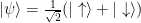
To illustrate this more precisely, and consider where we might hit some snags in this analysis, let’s look at a quantum superposition state,

$\vert \psi \rangle = \frac{1}{\sqrt{2}} (\vert\uparrow \rangle + \vert\downarrow \rangle)$ .

If we were to take everything we learned in university quantum mechanics courses at face value, we could easily recognize that, upon measurement, this state can be found in either the $\vert\uparrow \rangle$ or $\vert\downarrow \rangle$ state with equal probability. However, let us now turn our attention toward the Wigner’s friend scenario: image that Wigner has a friend inside a laboratory performing an experiment and Wigner himself is outside of the laboratory, positioned ideally as a superobserver (he can freely perform any and all quantum experiments on the laboratory from his vantage point). Going back to the superposition state above, it remains true that Wigner’s friend can observe either up or down states with 50% probability upon measurement. However, we also know that states must evolve unitarily. Wigner, still positioned outside of the laboratory, continues to observe a superposition of states with ill-defined measurement outcomes. Hence, a paradox, and one formed due to the fundamental assumption that quantum mechanics applies at all scales to all observers. This is the heart of the quantum measurement problem.

An illustration of the setup of the extended Wigner’s friend scenario, now including laboratories controlled by Charlie and Debbie with superobservers Alice and Bob. Charlie and Debbie make measurements on an entangled state, while Alice and Bob make measurements on the laboratories of Charlie and Debbie, respectively. Source: Kok-Wei Bong et al.

Now, let’s extend this scenario, taking our usual friends Alice and Bob as superobservers to two separate laboratories. Charlie, in the laboratory observed by Alice, has a system of spin-½ particles with an associated Hilbert space, while Debbie, in the laboratory observed by Bob, has her own system of spin-½ particles with an associated Hilbert space. Within their separate laboratories, they make measurements of the spins of the particles along the z-axis and record their results. Then Alice and Bob, still situated outside the laboratories of their respective friends, can make three different types of measurements on the systems, one of which they choose to perform randomly. First, Alice could look inside Charlie’s laboratory, view his measurement, and assign it to her own. Second, Alice could restore the laboratory to some previous state. Third, Alice could erase Charlie’s record of results and instead perform her own random measurement directly on the particle. Bob can perform the same measurements using Debbie’s laboratory.

With this setup, the new theorem then identifies a set of inequalities derived from Local Friendliness correlations, which are extended from those given by Bell’s Theorem and can be independently violated. The authors then concocted a proof-of-principle experiment, which relies on explicitly thinking of the friends Charlie and Debbie as qubits, rather than people. Using the three measurement settings and choosing systems of polarization-encoded photons, the photon paths are then the “friends” (the photon either takes Charlie’s path, Debbie’s path, or some superposition of the two). After running this experiment some thousands of times, the authors concluded that their Local Friendliness inequalities should be violated, implying that one of the three initial assumptions cannot be correct.

The primary difference between this work and Bell’s Theorem is that it contains no prior assumptions about the underlying determinism of reality, including any hidden variables that could be used to predetermine the outcomes of events. The theorem itself is therefore built upon assumptions strictly weaker than those of Bell’s inequalities, meaning that any violations would lead to strictly stronger conclusions. This paves a promising pathway for future questions and experiments about the nature of observation and measurement, narrowing down the large menu of interpretations of quantum mechanics. The question of which of the assumptions — absoluteness of observed events, locality, and no-superdeterminism — is incorrect is left as an open question. While the first two are widely used throughout physics, the assumption of no-superdeterminism digs down into the question of what measurement really means and what is classed as an observer. These points will doubtlessly be in contention as physicists continue to explore the oddities that quantum theory has to offer, but this new theorem offers promising results on the path to understanding the quirky quantum world.

Machine Learning The LHC ABC’s

Article Title: ABCDisCo: Automating the ABCD Method with Machine Learning

Authors: Gregor Kasieczka, Benjamin Nachman, Matthew D. Schwartz, David Shih

Reference: arxiv:2007.14400

When LHC experiments try to look for the signatures of new particles in their data they always apply a series of selection criteria to the recorded collisions. The selections pick out events that look similar to the sought after signal. Often they then compare the observed number of events passing these criteria to the number they would expect to be there from ‘background’ processes. If they see many more events in real data than the predicted background that is evidence of the sought after signal. Crucial to whole endeavor is being able to accurately estimate the number of events background processes would produce. Underestimate it and you may incorrectly claim evidence of a signal, overestimate it and you may miss the chance to find a highly sought after signal.

However it is not always so easy to estimate the expected number of background events. While LHC experiments do have high quality simulations of the Standard Model processes that produce these backgrounds they aren’t perfect. Particularly processes involving the strong force (aka Quantum Chromodynamics, QCD) are very difficult to simulate, and refining these simulations is an active area of research. Because of these deficiencies we don’t always trust background estimates based solely on these simulations, especially when applying very specific selection criteria.

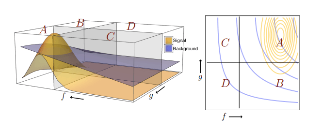
Therefore experiments often employ ‘data-driven’ methods where they estimate the amount background events by using control regions in the data. One of the most widely used techniques is called the ABCD method.

An illustration of the ABCD method. The signal region, A, is defined as the region in which f and g are greater than some value. The amount of background in region A is estimated using regions B C and D which are dominated by background.

The ABCD method can applied if the selection of signal-like events involves two independent variables f and g. If one defines the ‘signal region’, A, (the part of the data in which we are looking for a signal) as having f and g each greater than some amount, then one can use the neighboring regions B, C, and D to estimate the amount of background in region A. If the number of signal events outside region A is small, the number of background events in region A can be estimated as N_A = N_B * (N_C/N_D).

In modern analyses often one of these selection requirements involves the score of a neural network trained to identify the sought after signal. Because neural networks are powerful learners one often has to be careful that they don’t accidentally learn about the other variable that will be used in the ABCD method, such as the mass of the signal particle. If two variables become correlated, a background estimate with the ABCD method will not be possible. This often means augmenting the neural network either during training or after the fact so that it is intentionally ‘de-correlated’ with respect to the other variable. While there are several known techniques to do this, it is still a tricky process and often good background estimates come with a trade off of reduced classification performance.

In this latest work the authors devise a way to have the neural networks help with the background estimate rather than hindering it. The idea is rather than training a single network to classify signal-like events, they simultaneously train two networks both trying to identify the signal. But during this training they use a groovy technique called ‘DisCo’ (short for Distance Correlation) to ensure that these two networks output is independent from each other. This forces the networks to learn to use independent information to identify the signal. This then allows these networks to be used in an ABCD background estimate quite easily.

The authors try out this new technique, dubbed ‘Double DisCo’, on several examples. They demonstrate they are able to have quality background estimates using the ABCD method while achieving great classification performance. They show that this method improves upon the previous state of the art technique of decorrelating a single network from a fixed variable like mass and using cuts on the mass and classifier to define the ABCD regions (called ‘Single Disco’ here).

Using the task of identifying jets containing boosted top quarks, they compare the classification performance (x-axis) and quality of the ABCD background estimate (y-axis) achievable with the new Double DisCo technique (yellow points) and previously state of the art Single DisCo (blue points). One can see the Double DisCo method is able to achieve higher background rejection with a similar or better amount of ABCD closure.

While there have been many papers over the last few years about applying neural networks to classification tasks in high energy physics, not many have thought about how to use them to improve background estimates as well. Because of their importance, background estimates are often the most time consuming part of a search for new physics. So this technique is both interesting and immediately practical to searches done with LHC data. Hopefully it will be put to use in the near future!

Inside the Hologram

This is from arXiv:2009.04476 [hep-th] Inside the Hologram: Reconstructing the bulk observer’s experience

Figure 1 (adapted from arXiv:2009.04476 [hep-th]): The setup showing the reference system coupled to a black hole

The holographic principle in high energy physics has been proved to be quite rigorous. It has allowed physicists to understand phenomena that were too computationally difficult beforehand. The principle states that a theory describing gravity is related to a quantum theory. The gravity theory is typically called “the bulk” and the quantum theory is called “the boundary theory,” because it lives on the boundary of the gravity theory. Because the quantum theory is on the boundary, it is one dimension less than the gravity theory. Like a dictionary, physical concepts from gravity can be translated into physical concepts in the quantum theory. This idea of holography was introduced a few decades ago and a plethora of work has stemmed from it.

Much of the work regarding holography has been studied as seen from an asymptotic frame. This is a frame of reference that is “far away” from what we are studying, i.e. somewhere at the boundary where the quantum theory lives.

However, there still remains an open question. Instead of an asymptotic frame of reference, what about an internal reference frame? This is an observer inside the gravity theory, i.e. close to what we are studying. It seems that we do not have a quantum theory framework for describing physics for these reference frames. The authors of this paper explore this idea as they answer the question: how can we describe the quantum physics for an internal reference frame?

For classical physics, the usual observer is a probe particle. Since the authors want to understand the quantum aspects of the observer, they choose to have the observer be made up of a black hole that is entangled with a reference system. One way to see that black holes have quantum behavior is by studying Stephen Hawking’s work. Particularly, he showed that black hole can emit thermal radiation. This prediction is now known as Hawking radiation.

The authors proceed to measure the proper time between and energy distribution of the observer. Moreover, the researchers propose a new perspective on “time,” relating the notion of time in General Relativity to the notion of time in the quantum mechanics point of view, which may be valid outside the scope of holography.

The results have proven to be quite novel as it fills some of the gaps we have about our knowledge of holography. It is also a step towards understanding what the notion of time means in holographic gravitational systems.

September 25, 2020September 25, 2020

Catching The Higgs Speeding

Article Title: Inclusive search for highly boosted Higgs bosons decaying to bottom quark-antiquark pairs in proton-proton collisions at √s= 13 TeV

Authors: The CMS Collaboration

Reference arxiv:2006.13251

Since the discovery of the Higgs boson one of the main tasks of the LHC experiments has been to study all of its properties and see if they match the Standard Model predictions. Most of this effort has gone into characterizing the different ways the Higgs can be produced (‘production modes’) and how often it decays into its different channels (‘branching ratios’). However if you are a fan of Sonic the Hedgehog, you might have also wondered ‘How often does the Higgs go really fast?’. While that might sound like a very silly question, it is actually a very interesting one to study, and what has been done in this recent CMS analysis.

But what does it mean for the Higgs to ‘go fast’? You might have thought that the Higgs moves quite slowly because it is the 2nd heaviest fundamental particle we know of, with a mass around 125 times that of a proton. But sometimes very energetic LHC collisions can have enough energy to not only to make a Higgs boson but give it a ‘kick’ as well. If the Higgs is produced with enough momentum that it moves away from the beamline at a speed relatively close to the speed of light we call it ‘boosted’.

Not only are these boosted Higgs just a very cool thing to study, they can also be crucial to seeing the effects of new particles interacting with the Higgs. If there was a new heavy particle interacting with the Higgs during its production you would expect to see the largest effect on the rates of Higgs production at high momentum. So if you don’t look specifically at the rates of these boosted Higgs production you might miss this clue of new physics.

Another benefit is that when the Higgs is produced with a boost it significantly changes its experimental signature, often making it easier to spot. The Higgs’s favorite decay channel, its decay into a pair of bottom quarks, is notoriously difficult to study. A bottom quark, like any quark produced in an LHC collision, does not reach the detector directly, but creates a huge shower of particles known as a jet. Because bottom quarks live long enough to travel a little bit away from the beam interaction point before decaying, their jets start a little bit displaced compared to other jets. This allows experimenters to ‘tag’ jets likely to have come from bottom quarks. In short, the experimental signature of this Higgs decay is two jets that look bottom-like. This signal is very hard to find amidst a background of jets produced via the strong force which occur at rates orders of magnitude more often than Higgs production.

But when a particle with high momentum decays, its decay products will be closer together in the reference frame of the detector. When the Higgs is produced with a boost, the two bottom quarks form a single large jet rather than two separated jets. This single jet should have the signature of two b quarks inside of it rather than just one. What’s more, the distribution of particles within the jet should form 2 distinct ‘prongs’, one coming from each of the bottom quarks, rather than a single core that would be characteristic of a jet produced by a single quark or gluon. These distinct characteristics help analyzers pick out events more likely to be boosted Higgs from regular QCD events.

The end goal is to select events with these characteristics and then look for a excess of events that have an invariant mass of 125 GeV, which would be the tell-tale sign of the Higgs. When this search was performed they did see such a bump, an excess over the estimated background with a significance of 2.5 standard deviations. This is actually a stronger signal than they were expecting to see in the Standard Model. They measure the strength of the signal they see to be 3.7 ± 1.6 times the strength predicted by the Standard Model.

Higgs bump plot — The result of the search for ‘boosted’ Higgs bosons decaying to b quarks. One can see an excess of events at 125 GeV in pink corresponding to the observed Higgs signal

The analyzers then study this excess more closely by checking the signal strength in different regions of Higgs momentum. What they see is that the excess is coming from the events with the highest momentum Higgs’s. The significance of the excess of high momentum Higgs’s above the Standard Model prediction is about 2 standard deviations.

Higgs signal strength in different momentum bins — A plot showing the measured Higgs signal strength in different bins of the Higgs momentum. The signal strengths are normalized so the Standard Model prediction is always given by ‘1’ (shown in the gray dashed line. The measurement in each momentum bin are shown in the black points with red error bars. The overall measurement across all the bins is shown by the thick black line and the green region is the error bar.

So what we should we make of these extra speedy Higgs’s? Well first of all, the deviation from the Standard Model it is not very statistically significant yet, so it may disappear with further study. ATLAS is likely working on a similar measurement with their current dataset so we will wait to see if they confirm this excess. Another possibility is that the current predictions for the Standard Model, which are based on difficult perturbative QCD calculations, may be slightly off. Theorists will probably continue make improvements to these predictions in the coming years. But if we continue to see the same effect in future measurements, and the Standard Model prediction doesn’t budge, these speedy Higgs’s may turn out to be our first hint of the physics beyond the Standard Model!

SUSY vs. The Machines

Article title: Bayesian Neural Networks for Fast SUSY Predictions

Authors: B. S. Kronheim, M. P. Kuchera, H. B. Prosper, A. Karbo

Reference: https://arxiv.org/abs/2007.04506

It has been a while since we have graced these parts with the sounds of the attractive yet elusive superhero named SUSY. With such an arduous history of experimental effort, supersymmetry still remains unseen by the eyes of even the most powerful colliders. Though in the meantime, phenomenologists and theorists continue to navigate the vast landscape of model parameters with hopes of narrowing in on the most intriguing predictions – even connecting dark matter into the whole mess.

How vast you may ask? Well the ‘vanilla’ scenario, known as the Minimal Supersymmetric Standard Model (MSSM) – containing partner particles for each of those of the Standard Model – is chock-full of over 100 free parameters. This makes rigorous explorations of the parameter space not only challenging to interpret, but also computationally expensive. In fact, the standard practice is to confine oneself to a subset of the parameter space, using suitable justifications, and go ahead to predict useful experimental observables like collider production rates or particle masses. One of these popular motivations is known as the phenoneological MSSM (pMSSM), which reduces the huge parameter area to just less than 20 by assuming the absence of things like SUSY-driven CP-violation, flavour changing neutral currents (FCNCs) and differences between first and second generation SUSY particles. With this in the toolbox, computations become comparatively more feasible, with just enough complexity to make solid but interesting predictions.

But even coming from personal experience, these spaces can still be typically be rather tedious to work through – especially since many parameter selections are theoretically nonviable and/or in disagreement with previously well-established experimental observables, like the mass of the Higgs Boson. Maybe there is a faster way?

Machine learning has shared a successful history with a lot of high-energy physics applications, particularly those with complex dynamics like SUSY. One particularly useful application, at which machine learning is very accomplished at, is classification of points as excluded or not excluded based on searches at the LHC by ATLAS and CMS.

In the considered paper, a special type of Neural Network (NN) known as a Bayesian Neural Network (BNN) is used, which notably rely on probablistic certainty of classification rather than simply classifying a result as one thing or the other.

Figure 1: Your standard Neural Network (NN) shown in A has a single weight for each of its neuron connections (just represented by a number), learned from the training set. However, a Bayesian Neural Network (BNN) represented in B instead has a posterior distribution for each weight. When trained, it takes a prior distribution and applies Bayesian methods to obtain a posterior distribution. Taken from https://doi.org/10.3389/fninf.2019.00067.

In a typical NN there is a space of adjustable parameters (often called “features”) and a list of “targets” for the model to learn classification from. In this particular case, the model parameters are of course the features to learn from – these mainly include mass parameters for the different superparticles in the spectrum. These are mapped to three different predictions or targets that can be computed from these parameters:

The mass of the lightest, neutral Higgs Boson (the 125 GeV one)
The cross sections of processes involving the superpartners to the elecroweak guage bosons (typically called the neutralinos and charginos – I will let you figure out which ones are the charged and neutral ones)
Whether the point is actually valid or not (or maybe theoretically consistent is a better way to put it).

Of course there is an entire suite of programs designed to carry out these calculations, which are usually done point by point in the parameter space of the pMSSM, and hence these would be used to construct the training data sets for the algorithm to learn from – one data set for each of the predictions listed above.

But how do we know our model is trained properly once we have finished the learning process? There are a number of metrics that are very commonly used to determine whether a machine learning algorithm can correctly classify the results of a set of parameter points. The following table sums up the four different types of classifications that could be made on a set of data.

Table 1: Classifications for data given the predicted and actual results.

The typical measures employed using this table are the precision, recall and F1 score which are in practice readily defined as:

$P = \frac{TP}{TP+FP}, \quad R = \frac{TP}{TP+FN}, \quad F_1 = 2\frac{P \cdot R}{P+R}.$

In predicting the validity of points, the recall especially will tell us the fraction of valid points that will be correctly identified by the algorithm. For example, the metrics for this validity data set are shown in Table 2.

Table 2: Metrics for point validity data set. A point is valid from the classifier if it exceeds a cutoff of 0.5 in the first row, with a more relaxed 3 standard deviations in the second.

With a higher Recall but lower precision for the 3 standard deviation cutoff it is clear that points with a larger uncertainty will be classified as valid in this case. Such a scenario would be useful in calculating further properties like the mass spectrum, but not neccesarily as the best classifier.

Similarly with the data set used to compute cross sections, the standard deviation can be used for points where the predictions are quite uncertain. On average their calculations revealed just over 3% percent error with the actual value of the cross section. Not to be outdone, in calculating the Higgs boson mass, within 2 GeV deviation of 125 GeV, the precision of the BNN was found to be 0.926 with a recall of 0.997, showing that very few parameter points that are actually conistent with the light neutral Higgs will actually be removed.

In the end, our whole purpose was to provide reliable SUSY predictions at a fraction of the time. It is well known that NNs provide relatively fast calculation, especially when utilizing powerful hardware, and in this case could acheive up to over 16 million times faster in computing a single point than standard SUSY software! Finally, it is worth to note that neural networks are highly scalable and so predictions from the 19-dimensional pMSSM are but one of the possibilities for NNs in calculating SUSY observables.

Futher Reading

[1] Bayesian Neural Networks and how they differ from traditional NNs: https://towardsdatascience.com/making-your-neural-network-say-i-dont-know-bayesian-nns-using-pyro-and-pytorch-b1c24e6ab8cd

[2] More on machine learning and A.I. and its application to SUSY: https://arxiv.org/abs/1605.02797

August 27, 2020August 27, 2020

Representation and Discrimination in Particle Physics

Particle physics, like its overarching fields of physics and astronomy, has a diversity problem. Black students and researchers are severely underrepresented in our field, and many of them report feeling unsupported, unincluded, and undervalued throughout their careers. Although Black students enter into the field as undergraduates at comparable rates to white students, 8.5 times more white students than Black students enter PhD programs in physics¹. This suggests that the problem lies not in generating interest for the subject, but in the creation of an inclusive space for science.

This isn’t new information, although it has arguably not received the full attention it deserves, perhaps because everybody has not been on the same page. Before we go any further, let’s start with the big question: why is diversity in physics important? In an era where physics research is done increasingly collaboratively, the processes of cultivating talent across the social and racial spectrum is a strength that benefits all physicists. Having team members who can ask new questions or think differently about a problem leads to a wider variety of ideas and creativity in problem-solving approaches. It is advantageous to diversify a team, as the cohesiveness of the team often matters more in collaborative efforts than the talents of the individual members. While bringing on individuals from different backgrounds doesn’t guarantee the success of this endeavor, it does increase the probability of being able to tackle a problem using a variety of approaches. This is critical to doing good physics.

This naturally leads us to an analysis of the current state of diversity in physics. We need to recognize that physics is both subject to the underlying societal current of white supremacy and often perpetuates it through unconscious biases that manifest in bureaucratic structures, admissions and hiring policies, and harmful modes of unchecked communication. This is a roadblock to the accessibility of the field to the detriment of all physicists, as high attrition rates for a specific group suggests a loss of talent. But more than that, we should be striving to create departments and workplaces where all individuals and their ideas are values and welcomed. In order to work toward this, we need to:

Gather data: Why are Black students and researchers leaving the field at significantly higher rates? What is it like to be Black in physics?
Introspect: What are we doing (or not doing) to support Black students in physics classrooms and departments? How have I contributed to this problem? How has my department contributed to this problem? How can I change these behaviors and advocate for others?
Act: Often, well-meaning discussions remain just that — discussions. How can we create accountability to ensure that any agreed-upon action items are carried out? How can we track this progress over time?

Luckily, on the first point, there has been plenty of data that has already been gathered, although further studies are necessary to widen the scope of our understanding. Let’s look at the numbers.

Black representation at the undergraduate level is the lowest in physics out of all the STEM fields, at roughly 3%. This number has decreased from 5% in 1999, despite the total number of bachelor’s degrees earned in physics more than doubling during that time² (note: 13% of the United States population is Black). While the number of bachelor’s degrees earned by Black students increased by 36% across the physical sciences from 1995 to 2015, the corresponding percentage solely for physics degrees increased by only 4%². This suggests that, while access has theoretically increased, retention has not. This tells a story of extra barriers for Black physics students that push them away from the field.

This is corroborated as we move up the academic ladder. At the graduate level, the total number of physics PhDs awarded to Black students has fluctuated between 10 and 20 from 1997 to 2012⁴. From 2010 to 2012, only 2% of physics doctoral students in the United States were Black out of a total of 843 total physics PhDs⁴. For Black women, the numbers are the most dire, having received only 22 PhDs in astronomy and 144 PhDs in physics or closely-related fields in the entire history of United States physics graduate programs. Meanwhile, the percentage of Black faculty members from 2004 to 2012 has stayed relatively consistent, hovering around 2%⁵. Black students and faculty alike often report being the sole Black person in their department.

Where do these discrepancies come from? In January, the American Institute for Physics (AIP) released its TEAM-UP report summarizing what it found to be the main causes for Black underrepresentation in physics. According to the report, a main contribution to these numbers is whether students are immersed in a supportive environment². With this in mind, the above statistics are bolstered by anecdotal evidence and trends. Black students are less likely to report a sense of belonging in physics and more likely to report experiencing feelings of discouragement due to interactions with peers². They report lower levels of confidence and are less likely to view themselves as scientists². When it comes to faculty interaction, they are less likely to feel comfortable approaching professors and report fewer cases of feeling affirmed by faculty². Successful Black faculty describe gatekeeping in hiring processes, whereby groups of predominantly white male physicists are subject to implicit biases and are more likely to accept students or hire faculty who remind them of themselves³.

It is worth noting that this data comes in light of the fact that diversity programs have been continually implemented during the time period of the study. Most of these programs focus on raising awareness of a diversity problem, scraping at the surface instead of digging deeper into the foundations of this issue. Clearly, this approach has fallen short, and we must shift our efforts. The majority of diversity initiatives focus on outlawing certain behaviors, which studies suggest tends to reaffirm biased viewpoints and lead to a decrease in overall diversity⁶. These programs are often viewed as a solution in their own right, although it is clear that simply informing a community that bias exists will not eradicate it. Instead, a more comprehensive approach, geared toward social accountability and increased spaces for voluntary learning and discussion, might garner better results.

On June 10th, a team of leading particle physicists around the world published an open letter calling for a strike, for Black physicists to take a much-needed break from emotional heavy-lifting and non-Black physicists to dive into the self-reflection and conversation that is necessary for such a shift. The authors of the letter stressed, “Importantly, we are not calling for more diversity and inclusion talks and seminars. We are not asking people to sit through another training about implicit bias. We are calling for every member of the community to commit to taking actions that will change the material circumstances of how Black lives are lived — to work toward ending the white supremacy that not only snuffs out Black physicist dreams but destroys whole Black lives.”

“…We are calling for every member of the community to commit to taking actions that will change the material circumstances of how Black lives are lived — to work toward ending the white supremacy that not only snuffs out Black physicist dreams but destroys whole Black lives.” -Strike for Black Lives

Black academics, including many physicists, took to Twitter to detail their experiences under the hashtag #Blackintheivory. These stories painted a poignant picture of discrimination: being told that an acceptance to a prestigious program was only because “there were no Black women in physics,” being required to show ID before entering the physics building on campus, being told to “keep your head down” in response to complaints of discrimination, and getting incredulous looks from professors in response to requests for letters of recommendation. Microaggressions — brief and commonplace derisions, derogatory terms, or insults toward a group of people — such as these are often described as being poked repeatedly. At first, it’s annoying but tolerable, but over time it becomes increasingly unbearable. We are forcing Black students and faculty to constantly explain themselves, justify their presence, and prove themselves far more than any other group. While we all deal with the physics problem sets, experiments, and papers that are immediately in front of us, we need to recognize the further pressures that exist for Black students and faculty. It is much more difficult to focus on a physics problem when your society or department questions your right to be where you are. In the hierarchy of needs, it’s obvious which comes first.

Physicists, I’ve observed, are especially proud of the field they study. And rightfully so — we tackle some of the deepest, most fundamental questions the universe has to offer. Yet this can breed a culture of arrogance and “lone genius” stereotypes, with brilliant idolized individuals often being white older males. In an age of physics that is increasingly reliant upon large collaborations such as CERN and LIGO, this is not only inaccurate but actively harmful. The vast majority of research is done in teams, and creating a space where team members can feel comfortable is paramount to its success. Often, we can put on a show of being bastions of intellectual superiority, which only pushes away students who are not as confident in their abilities or who look around the room and see nobody else like them in it.

Further, some academics use this proclaimed superiority to argue their way around any issues of diversity and inclusion, choosing to see the data (such as GPA or test scores) without considering the context. Physicists tend to tackle problems in an inherently academic, systematic fashion. We often remove ourselves from consideration because we want physics to stick to a scientific method free from bias on behalf of the experimenter. Yet physics, as a human activity undertaken by groups of individuals from a society, cannot be fully separated from the society in which it is practiced. We need to consider: Who determines allocation of funding? Who determines which students are admitted, or which faculty are hired?

The TEAM-UP recommendations for increasing Black representation and cultivating a more welcoming environment in physics.

In order to fully transform the systems that leave Black students and faculty in physics underrepresented, unsupported, and even blatantly pushed out of the field, we must do the internal work as individuals and as departments to recognize harmful actions and put new systems in place to overturn these policies. With that in mind, what is the way forward? While there may be an increase in current momentum for action on this issue, it is critical to find a sustainable solution. This requires having difficult conversations and building accountability in the long term by creating or joining a working group within a department focused on equity, diversity, and inclusion (EDI) efforts. These types of fundamental changes are not possible without more widespread involvement; often, the burden of changing the system often falls on members of minority groups. The TEAM-UP report published several recommendations, centered on several categories including the creation of a resource guide, re-evaluating harassment response, and collecting data in an ongoing fashion. Further, Black scientists have long urged for the following actions⁷:

The creation of opportunities for discussion amongst colleagues on these issues. This could be accomplished through working groups or reading groups within departments. The key is having a space solely focused on learning more deeply about EDI.
Commitments to bold hiring practices, including cluster hiring. This occurs when multiple Black faculty members are hired at once, in order to decrease the isolation that occurs from being the sole Black member of a department.
The creation of a welcoming environment. This one is trickier, given that the phrase “welcoming environment” means something different to different people. An easier way to get a feel for this is by collecting data within a department, of both satisfaction and any personal stories or comments students or faculty would like to report. This also requires an examination of microaggressions and general attitudes toward Black members of a department, as an invite to the table could also be a case of tokenization.
A commitment to transparency. Research has shown that needing to explain hiring decisions to a group leads to a decrease in bias⁶.

While this is by no means a comprehensive list, there are concrete places for all of us to start.

References:

July 31, 2020July 31, 2020

First Evidence the Higgs Talks to Other Generations

Article Titles: “Measurement of Higgs boson decay to a pair of muons in proton-proton collisions at sqrt(S) = 13 TeV” and “A search for the dimuon decay of the Standard Model Higgs boson with the ATLAS detector”

Authors: The CMS Collaboration and The ATLAS Collaboration, respectively

References: CDS: CMS-PAS-HIG-19-006 and arxiv:2007.07830, respectively

Like parents who wonder if millennials have ever read a book by someone outside their generation, physicists have been wondering if the Higgs communicates with matter particles outside the 3rd generation. Since its discovery in 2012, phycists at the LHC experiments have been studying the Higgs in a variety of ways. However despite the fact that matter seems to be structured into 3 distinct ‘generations’ we have so far only seen the Higgs talking to the 3rd generation. In the Standard Model, the different generations of matter are 3 identical copies of the same kinds of particles, just with each generation having heavier masses. Due to the fact that the Higgs interacts with particles in proportion to their mass, this means it has been much easier to measure the Higgs talking to the third and heaviest generation of mater particles. But in order to test whether the Higgs boson really behaves exactly like the Standard Model predicts or has slight deviations -(indicating new physics), it is important to measure its interactions with particles from the other generations too. The 2nd generation particle the Higgs decays most often to is the charm quark, but the experimental difficulty of identifying charm quarks makes this an extremely difficult channel to probe (though it is being tried).

The best candidate for spotting the Higgs talking to the 2nd generation is by looking for the Higgs decaying to two muons which is exactly what ATLAS and CMS both did in their recent publications. However this is no easy task. Besides being notoriously difficult to produce, the Higgs only decays to dimuons two out of every 10,000 times it is produced. Additionally, there is a much larger background of Z bosons decaying to dimuon pairs that further hides the signal.

The branching ratio (fraction of decays to a given final state) of the Higgs boson as a function of its mass (the measured Higgs mass is around 125 GeV). The decay to a pair of muons is shown in gold, much below the other decays that have been observed.

CMS and ATLAS try to make the most of their data by splitting up events into multiple categories by applying cuts that target different the different ways Higgs bosons are produced: the fusion of two gluons, two vector bosons, two top quarks or radiated from a vector boson. Some of these categories are then further sub-divided to try and squeeze out as much signal as possible. Gluon fusion produces the most Higgs bosons, but it also the hardest to distinguish from the Z boson production background. The vector boson fusion process produces the 2nd most Higgs and is a more distinctive signature so it contributes the most to the overall measurement. In each of these sub-categories a separate machine learning classifier is trained to distinguish Higgs boson decays from background events. All together CMS uses 14 different categories of events and ATLAS uses 20. Backgrounds are estimated using both simulation and data-driven techniques, with slightly different methods in each category. To extract the overall amount of signal present, both CMS and ATLAS fit all of their respective categories at once with a single parameter controlling the strength of a Higgs boson signal.

At the end of the day, CMS and ATLAS are able to report evidence of Higgs decay to dimuons with a significance of 3-sigma and 2-sigma respectively (chalk up 1 point for CMS in their eternal rivalry!). Both of them find an amount of signal in agreement with the Standard Model prediction.

Combination of all the events used in the CMS (left) and ATLAS (right) searches for a Higgs decaying to dimuons. Events are weighted by the amount of expected signal in that bin. Despite this trick, the small evidence for a signal can be seen only be seen in the bottom panels showing the number of data events minus the predicted amount of background around 125 GeV.

CMS’s first evidence of this decay allows them to measuring the strength of the Higgs coupling to muons as compared to the Standard Model prediction. One can see this latest muon measurement sits right on the Standard Model prediction, and probes the Higgs’ coupling to a particle with much smaller mass than any of the other measurements.

CMS’s latest summary of Higgs couplings as a function of particle mass. This newest edition of the coupling to muons is shown in green. One can see that so far there is impressive agreement with the Standard Model across a mass range spanning 3 orders of magnitude!

As CMS and ATLAS collect more data and refine their techniques, they will certainly try to push their precision up to the 5-sigma level needed to claim discovery of the Higgs’s interaction with the 2nd generation. They will be on the lookout for any deviations from the expected behavior of the SM Higgs, which could indicate new physics!

Further Reading:

Older ATLAS Press Release “ATLAS searches for rare Higgs boson decays into muon pairs”

Cern Courier Article “The Higgs adventure: five years in”

Particle Bites Post “Studying the Higgs via Top Quark Couplings”

Blog Post from Matt Strassler on “How the Higgs Field Works“

July 26, 2020July 26, 2020

A simple matter

Article title: Evidence of A Simple Dark Sector from XENON1T Anomaly

Authors: Cheng-Wei Chiang, Bo-Qiang Lu

Reference: arXiv:2007.06401

As with many anomalies in the high-energy universe, particle physicists are rushed off their feet to come up with new, and often somewhat often complicated models to explain them. With the recent detection of an excess in electron recoil events in the 1-7 keV region from the XENON1T experiment (see Oz’s post in case you missed it), one can ask whether even the simplest of models can even still fit the bill. Although still at 3.5 sigma evidence – not quite yet in the ‘discovery’ realm – there is still great opportunity to test the predictability and robustness of our most rudimentary dark matter ideas.

The paper in question considers would could be one of the simplest dark sectors with the introduction of only two more fundamental particles – a dark photon and a dark fermion. The dark fermion plays the role of the dark matter (or part of it) which communicates with our familiar Standard Model particles, namely the electron, through the dark photon. In the language of particle physics, the dark sector particles actually carries a kind of ‘dark charge’, much like the electron carries what we know as the electric charge. The (almost massless) dark photon is special in the sense that it can interact with both the visible and dark sector – and as opposed to visible photons, and have a very long mean free path able to reach the detector on Earth. An important parameter describing how much the ordinary and dark photon ‘mix’ together is usually described by $\varepsilon$ . But how does this fit into the context of the XENON 1T excess?

Fig 1: Annihilation of dark fermions into dark photon pairs

The idea is that the dark fermions annihilate into pairs of dark photons (seen in Fig. 1) which excite electrons when they hit the detector material, much like a dark version of the photoelectric effect – only much more difficult to observe. The processes above remain exclusive, without annihilating straight to Standard Model particles, as long as the dark matter mass remains less than the lightest charged particle, the electron. With the electron at a few hundred keV, we should be fine in the range of the XENON excess.

What we are ultimately interested in is the rate at which the dark matter interacts with the detector, which in high-energy physics are highly calculable:

$\frac{d R}{d \Delta E}= 1.737 \times 10^{40}\left(f_{\chi} \alpha^{\prime}\right)^{2} \epsilon(E)\left(\frac{\mathrm{keV}}{m_{\chi}}\right)^{4}\left(\frac{\sigma_{\gamma}\left(m_{\chi}\right)}{\mathrm{barns}}\right) \frac{1}{\sqrt{2 \pi} \sigma} e^{-\frac{\left(E-m_{\chi}\right)^{2}}{2 \sigma^{2}}}$

where $f_{\chi}$ is the fraction of dark matter represented by $\chi$ , $\alpha'=\varepsilon e^2_{X} / (4\pi)$ , $\epsilon(E)$ is the efficiency factor for the XENON 1T experiment and $\sigma_{\gamma}$ is the photoelectric cross section.

Figure 2 shows the favoured regions for the dark fermion explanation fot the XENON excess. The dashed green lines represent only a 1% fraction of dark fermion matter for the universe, whilst the solid lines are to explain the entire dark matter content. Upper limits from the XENON 1T data is shown in blue, with a bunch of other astrophysical contraints (namely red giants, red dwarfs and horizontal branch star) far above the preffered regions.

Fig 2: The green bands represent the 1 and 2 sigma parameter regions in the $\alpha' - m_{\chi}$ plane favoured by the dark fermion model in explaning the XENON excess. The solid lines cover the entire DM component, whilst the dashed lines are only a 1% fraction.

Fig 2: The green bands represent the 1 and 2 sigma parameter regions in the $\alpha' - m_{\chi}$ plane favoured by the dark fermion model in explaning the XENON excess. The solid lines cover the entire DM component, whilst the dashed lines are only a 1% fraction.

This plot actually raises another important question: How sensitive are these results to the fraction of dark matter represented by this model? For that we need to specify how the dark matter is actually created in the first place – with the two most probably well-known mechanisms the ‘freeze-out’ and the ‘freeze-in’ (follow the links to previous posts!)

Fig 3: Freeze-out and freeze-in mechanisms for producing the dark matter relic density. The measured density (from PLANCK) is $\Omega h^2 = 0.12$ , shown on the red solid curve. The best fit values are also shown by the dashed lines, with their 1 sigma band. The mass of the dark fermion is fixed to its best-fit value of 3.17 keV, from Figure 2.

Fig 3: Freeze-out and freeze-in mechanisms for producing the dark matter relic density. The measured density (from PLANCK) is $\Omega h^2 = 0.12$ , shown on the red solid curve. The best fit values are also shown by the dashed lines, with their 1 sigma band. The mass of the dark fermion is fixed to its best-fit value of 3.17 keV, from Figure 2.

The first important point to note from the above figures is that the freeze-out mechanism doesn’t even depend on the mixing between the visible and dark sector i.e. the vertical axes. However, recall that the relic density in freeze-out is determined by the rate of annihlation into SM fermions – which is of course forbidden here for the mass of fermionic DM. The freeze-in works a little differently since there are two processes that can contribute to populating the relic density of DM: SM charged fermion annihlations and dark photon annihilations. It turns out that the charged fermion channel dominates for larger values of $e_X$ and in of course then becomes insensitive to the mixing parameter $\varepsilon$ and hence dark photon annihilations.

Of course it has been emphasized in previous posts that the only way to really get a good test of these models is with more data. But the advantage of simple models like these are that they are readily available in the physicist’s arsenal when anomalies like these pop up (and they do!)