ParticleBites summary – Page 3

September 4, 2014February 19, 2017

Neutrinoless Double Beta Decay Experiments

Title: Neutrinoless Double Beta Decay Experiments
Author: Alberto Garfagnini
Published: arXiv:1408.2455 [hep-ex]

Neutrinoless double beta decay is a theorized process that, if observed, would provide evidence that the neutrino is its own antiparticle. The relatively recent discovery of neutrino mass from oscillation experiments makes this search particularly relevant, since the Majorana mechanism that requires particles to be self-conjugate can also provide mass. A variety of experiments based on different techniques hope to observe this process. Before providing an experimental overview, we first discuss the theory itself.

DBD — Figure 1: Neutrinoless double beta decay.

Beta decay occurs when an electron or positron is released along with a corresponding neutrino. Double beta decay is simply the simultaneous beta decay of two neutrons in a nucleus. “Neutrinoless,” of course, means that this decay occurs without the accompanying neutrinos; in this case, the two neutrinos in the beta decay annihilate with one another, which is only possible if they are self-conjugate. Figures 1 and 2 demonstrate the process by formula and image, respectively.

doubleBetaandNeutrinoless — Figure 2: Double beta decay & neutrinoless double beta decay, from particlecentral.com/neutrinos_page.html.

The lack of accompanying neutrinos in such a decay violates lepton number, meaning this process is forbidden unless neutrinos are Majorana fermions. Without delving into a full explanation, this simply means that a particle is its own antiparticle (though more information is given in the references.) The importance lies in the lepton number of a neutrino. Neutrinoless double beta decay would require a nucleus to absorb two neutrinos, then decay into two protons and two electrons (to conserve charge). The only way in which this process does not violate lepton number is if the lepton charge is the same for a neutrino and an antineutrino; in other words, if they are the same particle.

The experiments currently searching for neutrinoless double beta decay can be classified according to the material used for detection. A partial list of active and future experiments is provided below.

1. EXO (Enriched Xenon Observatory): New Mexico, USA. The detector is filled with liquid ¹³⁶Xe, which provides worse energy resolution than gaseous xenon, but is compensated by the use of both scintillating and ionizing signals. The collaboration finds no statistically significant evidence for 0νββ decay, and place a lower limit on the half life of 1.1 * 10²⁵ years at 90% confidence.

2. KamLAND-Zen: Kamioka underground neutrino observatory near Toyama, Japan. Like EXO, the experiment uses liquid xenon, but in the past has required purification due to aluminum contaminations in the detector. They report a 0νββ half life 90% CL at 2.6 * 10²⁵years. Figure 3 shows the energy spectra of candidate events with the best fit background.

3. GERDA (Germanium Dectetor Array): Laboratori Nazionali del Gran Sasso, Italy. GERDA utilizes High Purity ⁷⁶Ge diodes, which provide excellent energy resolution but typically have very large backgrounds. To prevent signal contamination, GERDA has ultra-pure shielding that protect measurements from environmental radiation background sources. The half life is bound below at 90% confidence by 2.1 * 10²⁵ years.

4. MAJORANA: South Dakota, USA. This experiment is under construction, but a prototpye is expected to begin running in 2014. If results from GERDA and MAJORANA look good, there is talk of building a next generation germanium experiment that combines diodes from each detector.

5. CUORE: Laboratori Nazionali del Gran Sasso, Italy. CUORE is a ¹³⁰Te bolometric direct detector, meaning that it has two layers: an absorber made of crystal that releases energy when struck, and a sensor which detects the induced temperature changes. The experiment is currently under construction, so there are no definite results, but it expects to begin taking data in 2015.

While these results do not seem to show the existence of 0νββ decay, such an observation would demonstrate the existence of Majorana fermions and give an estimate of the absolute neutrino mass scale. However, a missing observation would be just as significant in the role of scientific discovery, since this would imply that the neutrino is not in fact its own antiparticle. To get a better limit on the half life, more advanced detector technologies are necessary; it will be interesting to see if MAJORANA and CUORE will have better sensitivity to this process.

Further Reading:

“Evidence for Neutrino Mass: A Decade of Discovery”: arXiv:0412032
“Recent Results in Neutrinoless Double Beta Decay”: arXiv:1305.3306
“Dirac, Majorana, and Weyl Fermions”: arXiv:1006.1718

September 2, 2014February 19, 2017

The Proton Radius Problem

The hydrogen atom is one of the primary examples studied in a typical introductory quantum mechanics course. Recent measurements indicate that this simple system may still have surprises for us. Could this be a hint of new physics? This post is based on the following papers:

“Muonic hydrogen and MeV forces” by D. Tucker-Smith and I. Yavin [1011.4922], Phys. Rev. D83 (2011) 101702

“Proton size anomaly” by V. Barger, C. Chiang, W. Keung, D. Marfatia [1011.3519], Phys. Rev. Lett. 106 (2011) 153001

“The Size of the Proton” by Pohl et al. in Nature 466 (2010) 213

Quantum mechanically, the proton is an object whose electric charge is smeared out over a small region. Experiments that scatter electrons off protons can probe this spatial extent and recent measurements indicate an effective proton charge radius of 0.877(7) femtometers.

Electron scattering experiments see a proton charge radius of 0.88 fm. — Electron scattering experiments measure a particular proton radius. (Image by the author.)

Muons are heavy copies of electrons and can similarly form muonic hydrogen: an atom formed from a proton and a muon. Because the muons are heavier, they exist closer to the nucleus and are more sensitive to the extent of the proton charge: the effective Coulomb force is reduced as one dips into the charge distribution in the same way that the gravitational force decreases as one digs towards the center of the Earth.

By ‘tickling’ the muon into a higher energy level with a laser and then measuring the resulting X-ray emission, one can deduce the proton radius. Since lasers can be tuned to very precise frequencies, one can make a very precise measurement of the Lamb shift in the muonic hydrogen energy levels. This, in turn, can be converted into a measurement of the proton radius because the energy levels are sensitive to the overlap of the muon and proton probability distributions. Intuitively, when the muon is inside the proton charge radius, it experiences a weaker Coulomb potential due to screening.

The big surprise is that the muonic hydrogen measurement gives a radius of 0.842(7) femtometers, this is over five standard deviations smaller than the expected result based on regular hydrogen!

Measurements of the proton charge radius from the lamb shift of muonic hydrogen (a proton--muon bound state) are smaller than that from electron scattering. — Measurements of the proton charge radius from the Lamb shift of muonic hydrogen are smaller than that from electron scattering by five standard deviations. (Image by the author)

This discrepancy remains an open question despite several proposed solutions based on more precise theoretical calculations to relate the Lamb shift to the proton radius. One optimistic approach is to entertain the possibility that this is an indicator of new fundamental physics, such as a heretofore undiscovered force that tugs on the muon and electron differently. It turns out that these types of models are difficult to construct. One of the main constraints is actually nearly 40 years old and comes from the effect of such a new force on neutron–lead scattering.

Meanwhile, a new set of experiments to probe the proton radius anomaly are already underway. One of these is the Muon-Proton Scattering Experiment (MUSE); this would directly probe if the origin of the discrepancy came from the two different proton radius measurements described above: scattering for electrons versus spectroscopy for muons.

CMS evidence of a possible SUSY decay chain

Title: “Search for physics beyond the standard model in events with two leptons, jets, and missing transverse energy in pp collisions at sqrt(s)=8 TeV.”
Author: CMS Collaboration
Published: CMS Public: Physics Results SUS12019

The CMS Collaboration, one of the two main groups working on multipurpose experiments at the Large Hadron Collider, has recently reported an excess of events with an estimated significance of 2.6σ. As a reminder, discoveries in particle physics are typically declared at 5σ. While this excess is small enough that it may not be related to new physics at all, it is also large enough to generate some discussion.

The excess occurs at an invariant mass of 20 – 70 GeV in dilepton + missing transverse energy (ME_T) decays. Some theorists claim that this may be a signature of supersymmetry. The analysis was completed using kinematic ‘edges’, an example of which can be seen in Figure 1. These shapes are typical of the decays of new particles predicted by supersymmetry.

edgeDiagram — Figure 1: Diagram of kinematic ‘edge’ effects in decay chains, from “Search for an ‘edge’ with CMS”. On the left, A, B, C, and D represent particles decaying. On the right, the invariant mass of final state particles C and D is shown, where the y axis represents the number of events.

The edge shape comes from the reconstructed invariant mass of the two leptons; in the diagram, these correspond to particles C and D. In models that conserve R-parity, which is the quantum number that distinguishes SUSY particles from Standard Model particles, a SUSY particle decays by emitting an SM particle and a lighter SUSY particle. In this case, two leptons are emitted in the chain. Reconstructing the invariant mass of the event is impossible because of the invisible massive particle. However, the total mass of the lepton pair can have any value, provided it is less than the maximum difference in mass between the initial and final state, as enforced by energy conservation. This maximum mass difference gives a hard cutoff, or ‘edge’, in the invariant mass distribution, as shown in the right side of Figure 1. Since the location of this cutoff is dependent on the mass of the original superparticle, these features can be very useful in obtaining information about such decays.

Figure 2 shows generated Monte Carlo for a new particle decaying to a two lepton final state. The red and blue lines show sources of background, while the green is the simulated signal. If the model was a good estimate of data, these three colored lines would sum to the distribution observed in data. Figure 3 shows the actual data distribution, with the relative significance of the excess around 20 – 70 GeV.

newSUSYMC — Figure 2: Monte Carlo invariant mass distribution of paired electrons or muons; signal shown in green with characteristic edge.

excessPlot — Figure 3: Invariant mass data distribution for paired leptons; excess between 20 and 70 GeV constitutes an estimated 2.6σ significance.

This excess is encouraging for physicists hoping to find stronger evidence for supersymmetry (or more generally, new physics) in Run II. However, 2.6σ is not especially high, and historically these excesses come and go all the time. Both CMS and ATLAS will certainly be watching this resonance in the 2015 13 TeV data, to see whether it grows into something more significant or simply fades into the background.

Further reading:

“Search for an ‘edge’ with CMS” explains the motivation for the analysis and shows additional plots.
A SUSY Edge Signal? CMS Sees A 2.6 Sigma Excess!
Supersymmetry Basics provides a good groundwork for how supersymmetry solves some current problems in particle physics.

August 15, 2014

New Results from the CRESST-II Dark Matter Experiment

Title: Results on low mass WIMPs using an upgraded CRESST-II detector
Author: G. Angloher, A. Bento, C. Bucci, L. Canonica, A. Erb, F. v. Feilitzsch, N. Ferreiro Iachellini, P. Gorla, A. Gütlein, D. Hauff, P. Huff, J. Jochum, M. Kiefer, C. Kister, H. Kluck, H. Kraus, J.-C. Lanfranchi, J. Loebell, A. Münster, F. Petricca, W. Potzel, F. Pröbst, F. Reindl, S. Roth, K. Rottler, C. Sailer, K. Schäffner, J. Schieck, J. Schmaler, S. Scholl, S. Schönert, W. Seidel, M. v. Sivers, L. Stodolsky, C. Strandhagen, R. Strauss, A. Tanzke, M. Uffinger, A. Ulrich, I. Usherov, M. Wüstrich, S. Wawoczny, M. Willers, and A. Zöller
Published: arXiv:1407.3146 [astro-ph.CO]

CRESST-II (Cryogenic Rare Event Search with Superconducting Thermometers) is a dark matter search experiment located at the Laboratori Nazionali del Gran Sasson in Italy. It is primarily involved with the search for WIMPs, or Weakly Interacting Massive Particles, which play a key role in both particle and astrophysics as a potential candidate for dark matter. If you are not yet intrigued enough about dark matter, see the list of references at the bottom of this post for more information. As dark matter candidates, WIMPs only interact via gravitational and weak forces, making them extremely difficult to detect.

CRESST-II attempts to detect WIMPs via elastic scattering off nuclei in scintillating CaWO4 crystals. This is a process known as direct detection, where scientists search for evidence of the WIMP itself; indirect detection requires searching for WIMP decay products. There are many challenges to direct detection, including the relatively low amount of recoil energy present in such scattering. An additional issue is the extremely high background, which is dominated by beta and gamma radiation of the nuclei. Overall, the experiment expects to obtain a few tens of events per kilogram-year.

CRESST1 — Figure 1: Expected number of events for background and signal in 2011 CRESST-II run; from 1109.0702v1.

In 2011, CREST-II reported a small excess of events outside of the predicted background levels. The statistical analysis makes use of a maximum likelihood function, which parameterizes each primary background to compute a total number of expected events. The results of this likelihood fit can be seen in Figure 1, where M1 and M2 are different mass hypotheses. From these values, CRESST-II reports a statistical significance of 4.7σ for M1, and 4.2σ for M2. Since a discovery is generally accepted to have a significance of 5σ, these numbers presented a pretty big cause for excitement.

In July of 2014, CRESST-II released a follow up paper: after some detector upgrades and further background reduction, these tantalizingly high significances have been revised, ruling out both mass hypotheses. The event excess was likely due to unidentified e^–/γ background, which was reduced by a factor of 2 -10 via improved CaWO4 crystals used in this run. The elimination of these high signal significances is in agreement with other dark matter searches, which have also ruled out WIMP masses on the order of 20 GeV.

Figure 2 shows the most recent exclusion curve for the WIMP mass, which gives the cross section for production as a function of possible mass. The contour reported in the 2011 paper is shown in light blue. The 90% confidence limit from the 2014 paper is given in solid red, alongside the expected sensivity from the background model in light red. All other curves are due to data from other experiments; see the paper cited for more information.

CRESST2 — Figure 2: WIMP parameter space for spin-independent WIMP-nucleon scattering, from 1407.3146v1.

Though this particular excess was ultimately not confirmed, these results overall present an optimistic picture for the dark matter search. Comparison between the limits from 2011 to 2014 show an much greater sensitivity for WIMP masses below 3 GeV, which were previously un-probed by other experiments. Additional detector improvements may result in even more stringent limit setting, shaping the dark matter search for future experiments.

Further Reading

June 12, 2014February 19, 2017

Black Holes enhance Dark Matter Annihilations

Title: Effect of Black Holes in Local Dwarf Spheroidal Galaxies on Gamma-Ray Constraints on Dark Matter Annihilation
Author: Alma X. Gonzalez-Morales, Stefano Profumo, Farinaldo S. Queiroz
Published: arXiv:1406.2424 [astro-ph.HE]

Upper bounds on dark matter annihilation from a combined analysis of 15 dwarf spheroidal galaxies for NFW (red) and Burkert (blue) DM density profiles. Fig. 4 from arXiv:1406.2424.

In a previous ParticleBite we showed how dwarf spheroidal galaxies can tell us about dark matter interactions. As a short summary, these are dark matter-rich “satellite [sub-]galaxies” of the Milky Way that are ideal places to look for photons coming from dark matter annihilation into Standard Model particles. In this post we highlight a recent update to that analysis.

The rate at which a pair of dark matter particles annihilate in a galaxy is proportional to the square of the dark matter density. The authors point out that if the dwarf spheroidal galaxies contain intermediate mass black holes ( $\sim 10^4$ times the mass of the sun), then its possible that the dark matter in the dwarf is more densely packed near the black hole. The authors redo the FERMI analysis for DM annihilation in dwarf spheroidals with 4 years of data (see our previous ParticleBite) with the assumption that these dwarfs contain a black hole consistent with their observed properties.

While the dwarf galaxies have little stellar content, one can use the visible stars to measure the stellar velocity dispersion, $\sigma_*$ . As a benchmark, the authors use the Tremaine relation to determine the black hole mass as a function of the observed velocity dispersion,

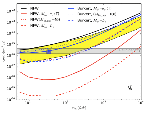
Here $M_{\odot}$ is the mass of the sun. Given this mass and its effect on the dark matter density, they can then calculate the J factor that encodes the `astrophysical’ line of slight integral of the squared dark matter density to observers on the Earth. Following the FERMI analysis, authors then set bounds on the dark matter annihilation cross section as a function of the dark matter mass for 15 dwarf spheroidals:

DM annihilation cross-section constraints for the b ̄b final state, for individual dSph, and for a combined analysis of 15 galaxies, assuming an initial NFW DM density distributio — DM annihilation cross-section constraints for annihilation into a pair of b quarks, from 1406.2424 Fig. 1. The shaded band is the target cross section to obtain the correct dark matter relic density through thermal freeze out, the red box is the target cross section for a dark matter interpretation of an excess in gamma rays in the galactic center.

Observe that the bounds are significantly stronger than those in the original FERMI analysis. In particular, the strongest bounds thoroughly rule out the “40 GeV DM annihilating into a pair of b quarks” interpretation of a reported excess in gamma rays coming from the galactic center. These bounds, however, come with several caveats that are described in the paper. The largest caveat is that the existence of a black hole in any of these systems is only assumed. The authors note that numerical simulations suggest that there should be black holes in these systems, but to date there has been no verification of their existence.

Further Reading

We refer to the previous ParticleBite for introductory material on indirect detection of dark matter.
See this blog post at io9 for a public-level exposition and video of observational evidence for the supermassive black hole (much heavier than the intermediate mass black holes posited in the dwarf spheroidals) at the center of the Milky Way.
See Ullio et al. (astro-ph/0101481) for an early paper describing the effect of black holes on the dark matter distribution.

June 5, 2014February 19, 2017

Dark Matter Shining from the Dwarfs

Title: Dark Matter Constraints from Observations of 25 Milky Way Satellite Galaxies with the Fermi Large Area Telescope
Author: FERMI-LAT Collaboration
Published: Phys.Rev. D89 (2014) 042001 [arXiv:1310.0828]

Dark matter (DM) is `dark’ because it does not directly interact with light. We suspect, however, that dark matter does interact with other Standard Model (SM) particles such as quarks and leptons. Since these SM particles do typically interact with photons, dark matter is indirectly luminous. More specifically, when two dark matter particles find each other and annihilate, their products include a spectrum photons that can be detected by telescopes. For typical `weakly-interacting massive particle’ DM candidates, these photons are in the GeV (γ-ray) range.

If dark matter interacts with the Standard Model, e.g. quarks, then its annihilation products include a spectrum of photons. Here we schematically show DM annihilating into quarks which shower into other colored `partons’ (quarks and gluons) that, in turn, become color-neutral hadrons. These then decay into light hadrons; the lightest of which (the neutral pion π) decays into two photons. Image adapted from D. Zeppenfeld (PiTP 05 lectures).

This type of indirect detection is a powerful handle to search for dark matter in the galaxy. The most promising place to search for these annihilation products are places where we expect a high density of dark matter, such as the galactic center. In fact, there have been recent hints for precisely this signal (see, e.g. this astrobite). Unfortunately, the galactic center is a very complicated environment with lots of other sources of GeV-scale photons that can make a DM interpretation tricky without additional checks.

Fortunately, there are other galactic objects that are dense with dark matter and have relatively little stellar (visible) matter: dwarf spheroidals. These satellite galaxies of the Milky Way are ideal laboratories for dark matter annihilation. While they have less dark matter density than the galactic center, they also have far fewer background photons from ordinary matter. Our tool of choice is the space-based Fermi-Large Area Telescope which is sensitive to photons between 0.03 — 300 GeV and surveys the entire sky every three hours.

Fig 1 of arXiv:1310.0828 — Map of known dwarf spheroidals over a ‘heat map’ of Fermi gamma-ray data. Image from 1310.0828.

The photon flux from dark matter annihilation is a product of three factors:

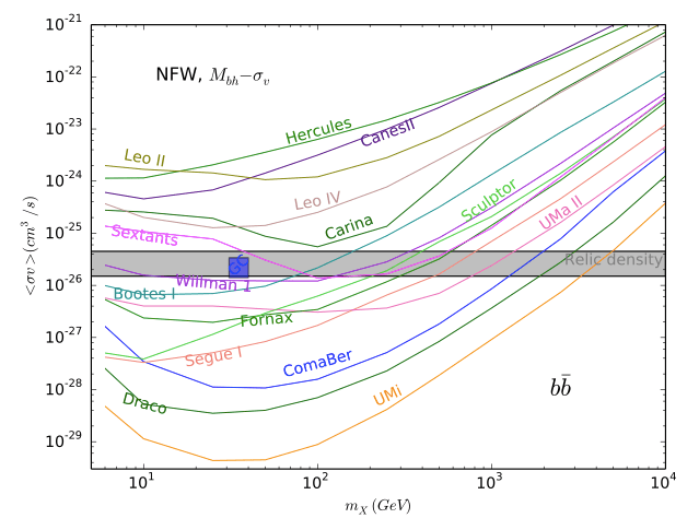
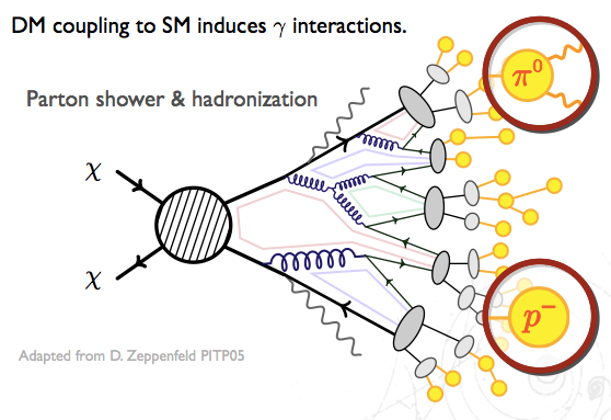
The “particle physics factor” describes the dark matter properties: its mass and annihilation rate. The $dN_\gamma/dE_\gamma$ factor describes the spectrum of photons coming from the DM annihilation products. The “astrophysics” factor is a line of sight integral along the dark matter density $\rho$ . Note that the $\rho^2$ from this factor and the $m_\chi^{-2}$ in the particle physics factor is simply the dark matter number density; the photon flux depends on how likely it is for DM particles to find each other. The astrophysics factor is sometimes called a J factor. For some of the dwarfs astronomers can determine the J factor based on the kinematics of the [few] stellar objects in the dwarf spheroidal.

One may use the morphology—or spatial distribution of dark matter—to help subtract background photons and fit data. For this ParticleBite we won’t discuss this step further except to emphasize that these fits are where all the astrophysics “muscle” enters. Each dwarf individually sets bounds on the dark matter profile, but one can combine (or “stack”) these results into a combined bound for each DM annihilation final state. The bounds differ depending on these annihilation products because each type of particle produces a different spectrum of photons that must be re-fit relative to the background. The dark matter mass controls the energy with which the ‘primary’ annihilation products are produced so that heavier dark matter masses yield more energetic photons.

blahblah — Combined dwarf spheroidal bounds on the annihilation cross section (roughly the rate of DM annihilation) as a function of the dark matter mass for a choice of DM annihilation products. Image from 1310.0828.

In the above plots, the green and yellow bands represent the approximate expected 1σ and 2σ sensitivity while the solid black line is the observed bound. There is a slight excess at lower masses, though the most optimistic excess in the b-quark channel has a significance of TS ~ 8.7, where TS is a ‘test statistic’ measure introduced in the paper. The relevant comparison is that TS ~ 25 is the standard Fermi uses for a discovery, so this excess should be understood to be fairly modest. (Note that the paper also notes that the statistical analysis underestimates statistical significance so that if one were to convert this into p-values or σ, one would overestimate the significance.)

Note further that the “stacked” analysis is most sensitive to those dwarfs with the largest J factors. Of these, half showed an excess while the other half were consistent with no excess.

The most important feature of the above plots is the horizontal dashed line. This line represents the dark matter annihilation cross section (“annihilation rate”) that one predicts based on the requirement that the observed dark matter density is set by this annihilation process. (There are ways around this, but it remains the simplest and most natural possibility.) The relevant bounds on the dark matter models, then, comes from looking at the point where the solid line and the dashed horizontal line meet. Dark matter masses to the left (i.e. less than) this value are disfavored in the simplest models.

For example, for dark matter that annihilates to b-quarks, one finds that the dwarf spheroidals set a lower limit on the dark matter mass of around 10 Gev. We note that this bound based on 4 years of Fermi data is weaker than the previously published 2 year results due, in part, to a revised analysis.

The future? A gamma ray excess in the galactic center (see, e.g. this astrobite) may possibly be interpreted as a signal of dark matter with mass of around 40 GeV annihilating into b quarks. At the moment the dwarf spheroidal bounds are to weak to probe this region. Will it ever? Since Fermi samples the entire sky, any newly identified dwarf spheroidal (e.g. from the Sloan Digital Sky Survey) automatically makes the full 4 year dataset for that dwarf available. Since the bounds scale like $\sqrt{N}$ (in the DM mass range below 200 GeV), one may roughly estimate the future sensitivity to the 40 GeV mass range as requiring 16 times more data. If we consider the next 4 years (doubling the observation time), this would require roughly 4 times more dwarfs to be identified. (See, e.g. this talk for a discussion.)

Further reading: some useful references for indirect detection of dark matter

September 30, 2013February 19, 2017

Fractional particles in the sky

Title: Goldstone Bosons as Fractional Cosmic Neutrinos

Author: Steven Weinberg (University of Texas, Austin)
Published: Phys.Rev.Lett. 110 (2013) 241301 [arXiv:1305.1971]

The Standard Model includes three types of neutrinos—the nearly-massless, charge-less partners of the leptons. Recent measurements from the Planck satellite, however, find that the ‘effective number of neutrinos’ in the early universe is $N_\text{eff} = 3.36 \pm 0.34$ . This is consistent with the Standard Model, but one may wonder what it means if this number really were fractional amount larger than three.

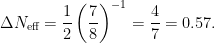
$fractionalneutrino$ Physically, $N_\text{eff}$ is actually a count of the number of light particles during recombination: the time in the early universe where the temperature had cooled enough for protons and electrons to form hydrogen. A snapshot era is imprinted on the cosmic microwave background (CMB). Particles whose masses are much less than the temperature—like neutrinos—are effectively ‘radiation’ during this era and affect the features of the CMB; see the appendix below for a rough sketch. In this way, cosmological observations can tell us about the spectrum of light particles.

The number $N_\text{eff}$ is defined as part of the ratio between photons and non-photon contributions to the ‘radiation’ density of the universe. It is normalized to count the number of light fermion–anti-fermion pairs. In this paper, Steven Weinberg points out that a light bosonic particle can give a fractional contribution to this counting. First of all, fermionic and bosonic contributions to the energy density differ by 7/8ths due to the difference between Fermi and Bose statistics. Secondly, a boson that is its own antiparticle picks up an additional 1/2, so that it looks like a light boson should contribute

$\displaystyle \Delta N_\text{eff} = \frac{1}{2} \left(\frac{7}{8}\right)^{-1} = \frac{4}{7} = 0.57.$

We have two immediate problems:

This is still larger than the observed mean that we’d like to hit, $\Delta N_\text{eff} = 0.36$ .
We’re implicitly assuming a new light scalar particle but quantum corrections generically make scalars very massive. (This is the essence of the Hierarchy problem associated with the Higgs mass.)

To address the second point, Weinberg assumes the new particle is a Goldstone boson—scalar particles which are naturally light because they’re associated with spontaneous symmetry breaking. For example, the lowest energy state of a ferromagnet breaks rotational symmetry since all the spins align in one direction. “Spin wave” excitations cost little energy and behave like light particles. Similarly, the strong force breaks chiral symmetry—which relates the behavior of left- and right-handed fermions. The pions are Goldstone bosons from this breaking and indeed have masses much smaller than other nuclear states like the proton. In this paper, Weinberg imagines that a new symmetry is broken spontaneously and the resulting Goldstone boson is the light state which can contribute to the number of light degrees of freedom in the early universe, $N_\text{eff}$ .

This set up also gives a way to address the first problem, how do we reduce the contribution of this particle, $\Delta N_\text{eff}$ , to better match what we observe in the CMB? One crucial assumption in our estimate for $\Delta N_\text{eff}$ was that the new light particle was in thermal equilibrium with neutrinos. As the universe cooled, the other Standard Model particles became too heavy to be produced thermally and their entropy had to go towards heating up the lighter particles. If the Goldstone boson fell out of thermal equilibrium too early—say, its interaction rate became too small to overcome the expanding distance between it and other particles—it won’t be heated by the heavy Standard Model particles. Because only the neutrinos are heated, the Goldstone contributes much less than 4/7 to $N_\text{eff}$ . (A sketch of the argument is in the appendix below.)

Weinberg points out that there’s an intermediate possibility: if the Goldstone boson just happens to go out of thermal equilibrium when only the muons, electrons, and neutrinos are still thermally accessible, then the only temperature increase for the neutrinos that isn’t picked up by the Goldstone comes from the muon. The expression for the entropy goes like

$\displaystyle s \sim T^3 \left(\text{Photon}\right) + \frac{7}{8} T^3 \left(\text{SM}\right)$

where “SM” refers to the number of Standard Model particles: a left-handed electron, a right-handed electron, a left-handed muon, a right-handed muon, and three left-handed neutrinos. (See this discussion on handedness.) The famous 7/8 shows up for the fermions. In order to conserve entropy when we lose the two muons, the other particles have to heat up by a factor of $ latex (57/43)^{1/3}$. Meanwhile, the Goldstone boson temperature stays constant since it doesn’t interact enough with the other particles to heat up. The contribution of the Goldstone to the effective number of light particles in the early universe is thus scaled down:

$\displaystyle \Delta N_\text{eff} = \frac{4}{7} \times \left(\frac{43}{57}\right)^{4/3} = 0.39,$

This is now quite close to the $\Delta N_\text{eff} = 0.36 \pm 0.34$ measured from the CMB. Weinberg goes on to construct an explicit example of how the Goldstone might interact with the Higgs to produce the correct interaction rates. As an example of further model building, he then notes that one may further construct models of dark matter where the broken symmetry that produced the Goldstone is associated with the stability of the dark matter particle.

Appendix

We briefly sketch how light particles can affect the cosmic microwave background. For details, see 1104.2333, the Snowmass paper 1309.5383, or the review in the PDG. Particles ‘decouple’ from the rest of the thermal particles in the early universe when their interaction rate is smaller than the expansion rate of the universe: the universe expands too quickly for the particles to stay in thermal equilibrium.

Neutrinos happen to decouple just before thermal electrons and positrons begin to annihilate. The energy from those annihilations thus go into heating the photons. From entropy conservation one can determine the fixed ratio between the neutrino and photon temperatures. This, in turn, allows one to determine the relative number and energy densities.

Additional contributions to the effective number of light particles $N_\text{eff}$ thus lead to an increase in the energy density. In the radiation dominated era of the universe, this increases the expansion rate (Hubble parameter). One can then use two observables to pin down the additional contribution to $N_\text{eff}$ .

CMB with the sound horizon $\theta_s$ and diffusion scale $\theta_d$ illustrated. Image from Lloyd Knox.

CMB with the sound horizon $\theta_s$ and diffusion scale $\theta_d$ illustrated. Image from Lloyd Knox.

Tension between gravitational pull and pressure from radiation produces acoustic oscillations in the microwave background. Two features which are sensitive to the Hubble parameter are:

The sound horizon. This is the scale of acoustic oscillations and can be seen in the peaks of the CMB power spectrum. The angular sound scale goes like $1/H$ .
The diffusion scale. This measures the damping of small scale oscillations from photons diffusion. This scale goes like $\sqrt{1/H}$ .

A heuristic picture of what these scales correspond to is shown if the figure. The measurement of these two parameters thus gives a fit for the Hubble parameter that can then give a fit for the effective number of light particles in the early universe, $N_\text{eff}$ .