It was that time of year again when the entire string theory community comes together to discuss current research programs, the status of string theory and more recently, the social issues common in the field. This annual conference has been held in various countries but for the first time in its 35 year-long history has been hosted in Latin America at the ICTP South American Institute for Fundamental Research (ICTP-SAIFR).
One positive aspect of its virtual platform has been the increase in the number of participants attending the conference. Similar to Strings 2020 held in South Africa, more than two thousand participants were registered for the conference. In addition to research talks on technical subtopics, participants were involved in daily informal discussions on topics such as the black hole information paradox, ensemble averaging, and cosmology and string theory. More junior participants were involved in the poster sessions and gong shows, held in the first week of the conference.
One particular discussion session I would like to point out was panel discussion on the 4 generations of women in string theory, featuring women from different age groups and how they have dealt with issues of gender and implicit bias in their current or previous roles in academia.
To say the very least, the conference was a major success and has shown the effectiveness of virtual platforms for upcoming years, possibly including Strings 2022 to be held in Vienna.
For the string theory enthusiasts reading this, recordings of the conference can be found here.
“Is N=2 large?” queried Kitano, Yamada and Yamazaki in their paper title. Exactly five months later, they co-wrote with Matsudo a paper titled “N=2 is large“, proving that their question was, after all, rhetorical.
Papers ask the darndest things. Collected below are titular posers from the field’s literature that keep us up at night.
Figure 1: a torus is an example of a geometry that has T-duality
Physicists have been searching for ways to describe the interplay between gravity and quantum mechanics – quantum gravity – for the last century. The problem of finding a consistent theory of quantum gravity still looms physicists to this day. Fortunately, string theory is the most promising candidate for such a task.
One of the strengths of string theory is that at low energies, the equations arising from string theory are shown to be precisely Einstein’s theory of general relativity. Let’s break down what this means. First, we must make sure we know the definition of a coupling constant. Theories of physics are typically described by some parameter that signifies the strength of the interaction. This parameter is called the coupling constant of that theory. According to quantum field theory, the value of the coupling constant depends on the energy. We often plot the logarithm of the energy and the coupling constant to understand how the theory behaves at a certain energy scale. The slope of this plot is called the beta function and when this function is zero, that point is called a fixed point. These fixed points are interesting since they imply that the quantum theory does not have any notion of scale.
Back to string theory, its coupling constant is called α′ (said as alpha-prime). At weak coupling, when α′ is small, we can similarly find the beta function for string theory. At the quantum level, string theory must have a vanishing beta function. At the corresponding fixed point, we find that the Einstein’s equations of motion emerge. This is quite remarkable!
We can go even further. Due to the smallness of α′, we can expand the beta function perturbatively. All the subleading terms in α′, which are infinite in number, are considered to be corrections to general relativity. Therefore, we can understand how general relativity is modified via string theory. It becomes technically challenging to compute these corrections and little is known about what the full expansion looks like.
Fortunately for physicists, string theories are interesting in other ways that could help figure us out these corrections to gravity. Particularly, the string energy spectrum that has radii R and radii α′/R look exactly the same. This relation is called T-duality. An example of a geometry that has this duality is the torus, see Figure 1. Because we know that certain dualities for strings must hold, we can use this to guess what the higher order correction must look like. Codina, Hohm and Marques took advantage of this idea to find corrections to the third power of α′. Using a simple scenario where the graviton is the only field in the theory, they were able to predict what the corrections must be.
This method can be applied at higher orders in α′ as well as a theory with more fields than the graviton, although technical challenges still arise. Due to the structure of how T-duality was used, the authors can also use their results to study cosmological models. Finally, the theory result confirms that string theory should be T-duality at all orders of α′.
Title : New physics and tau g−2 using LHC heavy ion collisions
Authors: Lydia Beresford and Jesse Liu
Reference: https://arxiv.org/abs/1908.05180
Since April, particle physics has been going crazy with excitement over the recent announcement of the muon g-2 measurement which may be our first laboratory hint of physics beyond the Standard Model. The paper with the new measurement has racked up over 100 citations in the last month. Most of these papers are theorists proposing various models to try an explain the (controversial) discrepancy between the measured value of the muon’s magnetic moment and the Standard Model prediction. The sheer number of papers shows there are many many models that can explain the anomaly. So if the discrepancy is real, we are going to need new measurements to whittle down the possibilities.
Given that the current deviation is in the magnetic moment of the muon, one very natural place to look next would be the magnetic moment of the tau lepton. The tau, like the muon, is a heavier cousin of the electron. It is the heaviest lepton, coming in at 1.78 GeV, around 17 times heavier than the muon. In many models of new physics that explain the muon anomaly the shift in the magnetic moment of a lepton is proportional to the mass of the lepton squared. This would explain why we are a seeing a discrepancy in the muon’s magnetic moment and not the electron (though there is a actually currently a small hint of a deviation for the electron too). This means the tau should be 280 times more sensitive than the muon to the new particles in these models. The trouble is that the tau has a much shorter lifetime than the muon, decaying away in just 10-13 seconds. This means that the techniques used to measure the muons magnetic moment, based on magnetic storage rings, won’t work for taus.
Thats where this new paper comes in. It details a new technique to try and measure the tau’s magnetic moment using heavy ion collisions at the LHC. The technique is based on light-light collisions (previously covered on Particle Bites) where two nuclei emit photons that then interact to produce new particles. Though in classical electromagnetism light doesn’t interact with itself (the beam from two spotlights pass right through each other) at very high energies each photon can split into new particles, like a pair of tau leptons and then those particles can interact. Though the LHC normally collides protons, it also has runs colliding heavier nuclei like lead as well. Lead nuclei have more charge than protons so they emit high energy photons more often than protons and lead to more light-light collisions than protons.
A Feynman diagram showing an “ultraperipheral collision” (UPC) between two lead nuclei. Both lead nuclei emit a photon and those two photons interact to produce two tau leptons that then decay.
Light-light collisions which produce tau leptons provide a nice environment to study the interaction of the tau with the photon. A particles magnetic properties are determined by its interaction with photons so by studying these collisions you can measure the tau’s magnetic moment.
However studying this process is be easier said than done. These light-light collisions are “Ultra Peripheral” because the lead nuclei are not colliding head on, and so the taus produced generally don’t have a large amount of momentum away from the beamline. This can make them hard to reconstruct in detectors which have been designed to measure particles from head on collisions which typically have much more momentum. Taus can decay in several different ways, but always produce at least 1 neutrino which will not be detected by the LHC experiments further reducing the amount of detectable momentum and meaning some information about the collision will lost.
However one nice thing about these events is that they should be quite clean in the detector. Because the lead nuclei remain intact after emitting the photon, the taus won’t come along with the bunch of additional particles you often get in head on collisions. The level of background processes that could mimic this signal also seems to be relatively minimal. So if the experimental collaborations spend some effort in trying to optimize their reconstruction of low momentum taus, it seems very possible to perform a measurement like this in the near future at the LHC.
Precision of the measurements of the anomalous magnetic moment of different leptons. The current best measurement of the tau’s anomalous magnetic moment is the DELPHI one with blue error bars, electron and muon measurements are the first two bars and are much more precise than that of the tau so their error bars have to been inflated to be visible. The green bars show the projected sensitivity using this new technique with different amounts of data and projections for the systematic uncertainty. The orange bar shows the value of the tau magnetic moment in some BSM scenarios that are compatible with current data.
The authors of this paper estimate that such a measurement with a the currently available amount of lead-lead collision data would already supersede the previous best measurement of the taus anomalous magnetic moment and further improvements could go much farther. Though the measurement of the tau’s magnetic moment would still be far less precise than that of the muon and electron, it could still reveal deviations from the Standard Model in realistic models of new physics. So given the recent discrepancy with the muon, the tau will be an exciting place to look next!
Title: Annual Modulation Results from Three Years Exposure of ANAIS-112.
Reference: https://arxiv.org/abs/2103.01175.
This is an exciting couple of months to be a particle physicist. The much-awaited results from Fermilab’s Muon g-2 experiment delivered all the excitement we had hoped for. (Don’t miss our excellent theoretical and experimental refreshers by A. McCune and A. Frankenthal, and the post-announcement follow-up.) Not long before that, the LHCb collaboration confirmed the flavor anomaly, a possible sign of violation of lepton universality, and set the needle at 3.1 standard deviations off the Standard Model (SM). That same month the ANAIS dark matter experiment took on the mighty DAMA/LIBRA, the subject of this post.
In its quest to confirm or refute its 20 year-old predecessor at Brookhaven National Lab, the Fermilab Muon g-2 experiment used the same storage ring magnet — though refurbished — and the same measurement technique. As the April 7 result is consistent with the BNL measurement, this removes much doubt from the experimental end of the discrepancy, although of course, unthought-of correlated systematics may lurk. A similar philosophy is at work with the ANAIS experiment, which uses the same material, technique and location (on the continental scale) as DAMA/LIBRA.
As my colleague M. Talia covers here and I touch upon here, an isotropic distribution of dark matter velocities in the Galactic frame would turn into an anisotropic “wind” in the solar frame as the Solar System orbits around the center of the Milky Way. Furthermore, in the Earth’s frame the wind would reverse direction every half-year as we go around the Sun. If we set up a “sail” in the form of a particle detector, this annual modulation could be observed — if dark matter interacts with SM states. The amplitude of this modulation is given by
where
is the rate of event collection per unit mass of detector per unit energy of recoil at some time ,
,
captures any unmodulated rate in the detector with its probability distribution in time, and
is fixed by the start date of the experiment so that the event rate is highest when we move maximally upwind on June 02.
The DAMA/LIBRA experiment in Italy’s Gran Sasso National Laboratory, using 250 kg of radiopure thallium-doped sodium-iodide [NaI(Tl)] crystals, claims to observe a modulation every year over the last 20 years, with /day/kg/keV in the 2–6 keV energy range at the level of .
It is against this serious claim that the experiments ANAIS, COSINE, SABRE and COSINUS have mounted a cross-verification campaign. Sure, the DAMA/LIBRA result is disfavored by conventional searches counting unmodulated dark matter events (see, e.g. Figure 3 here or this recent COSINE-100 paper). But it cannot get cleaner than a like-by-like comparison independent of assumptions about dark matter pertaining either to its microscopic behavior or to its phase space distribution in the Earth’s vicinity. Doing just that, ANAIS (for Annual Modulation with NaI Scintillators) in Spain’s Canfranc Underground Laboratory, using 112.5 kg of radiopure NaI(Tl) over 3 years, has a striking counter-claim summed up in this figure:
Figure caption: The ANAIS 3 year dataset is consistent with no annual modulation, in tension with DAMA’s observation of significant modulation over 20 years.
ANAIS’ error bars are unsurprisingly larger than DAMA/LIBRA’s given their smaller dataset, but the modulation amplitude they measure is unmistakably consistent with zero and far out from DAMA/LIBRA. The plot below is visual confirmation of non-modulation with the label indicating the best-fit under the modulation hypothesis.
Figure caption: ANAIS-112 event rate data in two energy ranges, fitted to a null hypothesis and a modulation hypothesis; the latter gives a fit consistent with zero modulation. The event rate here falls with time as the time-distribution of the background is modeled as an exponential function accounting for isotopic decays in the target material.
The ANAIS experimenters carry out a few neat checks of their result. The detector is split into 9 pieces, and just to be sure of no differences in systematics and backgrounds among them, every piece is analyzed for a modulation signal. Next they treat as a free parameter, equivalent to making no assumptions about the direction of the dark matter wind. Finally they vary the time bin size in analyzing the event rate such as in the figure above. In every case the measurement is consistent with the null hypothesis.
Exactly how far away is the ANAIS result from DAMA/LIBRA? There are two ways to quantify it. In the first, ANAIS take their central values and uncertainties to compute a 3.3 (2.6 ) deviation from DAMA/LIBRA’s central values in the 1–6 keV (2–6 keV) bin. In the second way, the ANAIS uncertainty is directly compared to DAMA using the ratio , giving 2.5 and 2.7 in those energy bins. With 5 years of data — as scheduled for now — this latter sensitivity is expected to grow to 3 . And with 10 years, it could get to 5 — and we can all go home.
Further reading.
[1] Watch out for the imminent results of the KDK experiment set out to study the electron capture decay of potassium-40, a contaminant in NaI; the rate of this background has been predicted but never measured.
[2] The COSINE-100 experiment in Yangyang National Lab, South Korea (note: same hemisphere as DAMA/LIBRA and ANAIS) published results in 2019 using a small dataset that couldn’t make a decisive statement about DAMA/LIBRA, but they are scheduled to improve on that with an announcement some time this year. Their detector material, too, is NaI(Tl).
[3] The SABRE experiment, also with NaI(Tl), will be located in both hemispheres to rule out direction-related systematics. One will be right next to DAMA/LIBRA at the Gran Sasso Laboratory in Italy, the other at Stawell Underground Physics Laboratory in Australia. ParticleBites’ M. Talia is excited about the latter.
[4] The COSINUS experiment, using undoped NaI crystals in Gran Sasso, aims to improve on DAMA/LIBRA by lowering the nuclear recoil energy threshold and with better background discrimination.
This is the final post of a three-part series on the Muon g-2 experiment. Check out posts 1 and 2 on the theoretical and experimental aspects of g-2 physics.
The last couple of weeks have been exciting in the world of precision physics and stress tests of the Standard Model (SM). The Muon g-2 Collaboration at Fermilab released their very first results with a measurement of the anomalous magnetic moment of the muon to an accuracy of 462 parts per billion (ppb), which largely agrees with previous experimental results and amplifies the tension with the accepted theoretical prediction to a 4.2 discrepancy. These first results feature less than 10% of the total data planned to be collected, so even more precise measurements are foreseen in the next few years.
But on the very same day that Muon g-2 announced their results and published their main paper on PRL and supporting papers on Phys. Rev. A and Phys. Rev. D, Nature published a new lattice QCD calculation which seems to contradict previous theoretical predictions of the g-2 of the muon and moves the theory value much closer to the experimental one. There will certainly be hot debate in the coming months and years regarding the validity of this new calculation, but it does not stop from muddying the waters in the g-2 sphere. We cover both the new experimental and theoretical results in more detail below.
Experimental announcement
The main paper in Physical Review Letters summarizes the experimental method and reports the measured numbers and associated uncertainties. The new Fermilab measurement of the muon g-2 is 3.3 standard deviations () away from the predicted SM value. This means that, assuming all systematic effects are accounted for, the probability that the null hypothesis (i.e. that the true muon g-2 number is actually the one predicted by the SM) could result in such a discrepant measurement is less than 1 in 1,000. Combining this latest measurement with the previous iteration of the experiment at Brookhaven in the early 2000s, the discrepancy grows to 4.2, or smaller than 1 in 300,000 probability that it is just a statistical fluke. This is not yet the 5 threshold that seems to be the golden standard in particle physics to claim a discovery, but it is a tantalizing result. The figure below from the paper illustrates well the tension between experiment and theory.
Comparison between experimental measurements of the anomalous magnetic moment of the muon (right, top to bottom: Brookhaven, Fermilab, combination) and the theoretical prediction by the Standard Model (left). The discrepancy has grown to 4.2 sigma. Source: https://journals.aps.org/prl/pdf/10.1103/PhysRevLett.126.141801
This first publication is just the first round of results planned by the Collaboration, and corresponds to less than 10% of the data that will be collected throughout the total runtime of the experiment. With this limited dataset, the statistical uncertainty (434 ppb) dominates over the systematic uncertainty (157 pbb), but that is expected to change as more data is acquired and analyzed. When the statistical uncertainty eventually dips below, it will be critically important to control the systematics as much as possible, to attain the ultimate target goal of a 140 ppb total uncertainty measurement. The table below shows the actual measurements performed by the Collaboration.
Table of measurements for each sub-run of the Run-1 period, from left to right: precession frequency, equivalent precession frequency of a proton (i.e. measures the magnetic field), and the ratio between the two quantities. Source: https://journals.aps.org/prl/pdf/10.1103/PhysRevLett.126.141801
The largest sources of systematic uncertainties stem from the electrostatic quadrupoles (ESQ) in the experiment. While the uniform magnetic field ensures the centripetal motion of muons in the storage ring, it is also necessary to keep them confined to the horizontal plane. Four sets of ESQ uniformly spaced in azimuth provide vertical focusing of the muon beam. However, after data-taking, two resistors in the ESQ system were found to be damaged. This means that the time profile of ESQ activation was not perfectly matched to the time profile of the muon beam. In particular, during the first 100 microseconds after each muon bunch injection, muons were not getting the correct focusing momentum, which affected the expected phase of the “wiggle plot” measurement. All told, this issue added 75 ppb of systematic uncertainty to the budget. Nevertheless, because statistical uncertainties dominate in this first stage of the experiment, the unexpected ESQ damage was not a showstopper. The Collaboration expects this problem to be fully mitigated in subsequent data-taking runs.
To guard against any possible human bias, an interesting blinding policy was implemented: the master clock of the entire experiment was shifted by an unknown value, chosen by two people outside the Collaboration and kept in a vault for the duration of the data-taking and processing. Without knowing this shift, it is impossible to deduce the correct value of the g-2. At the same time, this still allows experimenters to carry out the analysis through the end, and only then remove the clock shift to reveal the unblinded measurement. In a way this is like a key unlocking the final result. (This was not the only protection against bias, only the more salient and curious one.)
Lattice QCD + BMW results
On the same day that Fermilab announced the Muon g-2 experimental results, a group known as the BMW (Budapest-Marseille-Wuppertal) Collaboration published its own results on the theoretical value of muon g-2 using new techniques in lattice QCD. The group’s results can be found in Nature (the journal, jury’s still out on whether they’re in actual Nature), or at the preprint here. In short, their calculations bring them much closer to the experimental value than previous collaborations, bringing their methods into tension with the findings of previous lattice QCD groups. What’s different? To this end, let’s dive a little deeper into the details of lattice QCD.
The BMW group published this plot, showing their results (top line) compared with the results of other groups using lattice QCD (remaining green squares) and the R-ratio (the usual data-driven techniques, red circles). The purple bar gives the range of values for the anomalous magnetic moment that would signal no new physics – we can see that the BMW results are closer to this region than the R-ratio results, which have similarly small error bars. Source: BMW Collaboration
As outlined in the first post of this series, the main tool of high-energy particle physics rests in perturbation theory, which we can think of graphically via Feynman diagrams, starting with tree-level diagrams and going to higher orders via loops. Equivalently, this corresponds to calculations in which terms are proportional to some coupling parameter that describes the strength of the force in question. Each higher order term comes with one more factor of the relevant coupling, and our errors in these calculations are generally attributable to either uncertainties in the coupling measurements themselves or the neglecting of higher order terms.
These coupling parameters are secretly functions of the energy scale being studied, and so at each energy scale, we need to recalculate these couplings. This makes sense intuitively because forces have different strengths at different energy scales — e.g. gravity is much weaker on a particle scale than a planetary one. In quantum electrodynamics (QED), for example, these couplings are fairly small when in the energy scale of the electron. This means that we really don’t need to go to higher orders in perturbation theory, since these terms quickly become irrelevant with higher powers of this coupling. This is the beauty of perturbation theory: typically, we need only consider the first few orders, vastly simplifying the process.
However, QCD does not share this convenience, as it comes with a coupling parameter that decreases with increasing energy scale. At high enough energies, we can indeed employ the wonders of perturbation theory to make calculations in QCD (this high-energy behavior is known as asymptotic freedom). But at lower energies, at length scales around that of a proton, the coupling constant is greater than one, which means that the first-order term in the perturbative expansion is the least relevant term, with higher and higher orders making greater contributions. In fact, this signals the breakdown of the perturbative technique. Because the mass of the muon is in this same energy regime, we cannot use perturbation theory in quantum field theory to calculate g-2. We then turn to simulations, and since cannot entirely simulate spacetime (because it consists of infinite points), we must instead break it up into a discretized set of points dubbed the lattice.
A visualization of the lattice used in simulations. Particles like quarks are placed on the points of the lattice, with force-carrying gauge bosons (in this case, gluons) forming the links between them. Source: Lawrence Livermore National Laboratory
This naturally introduces new sources of uncertainty into our calculations. To employ lattice QCD, we need to first consider which lattice spacing to use — the distance between each spacetime point — where a smaller lattice spacing is preferable in order to come closer to a description of spacetime. Introducing this lattice spacing comes with its own systematic uncertainties. Further, this discretization can be computationally challenging, as larger numbers of points quickly eat up computing power. Standard numerical techniques become too computationally expensive to employ, and so statistical techniques as well as Monte Carlo integration are used instead, which again introduces sources of error.
Difficulties are also introduced by the fact that a discretized space does not respect the same symmetries that a continuous space does, and some symmetries simply cannot be kept simultaneously with others. This leads to a challenge in which groups using lattice QCD must pick which symmetries to preserve as well as consider the implications of ignoring the ones they choose not to simulate. All of this adds up to mean that lattice QCD calculations of g-2 have historically been accompanied by very large error bars — that is, until the much smaller error bars from the BMW group’s recent findings.
These results are not without controversy. The group employs a “staggered fermion” approach to discretizing the lattice, in which a single type of fermion known as a Dirac fermion is put on each lattice point, with additional structure described by neighboring points. Upon taking the “continuum limit,” or the limit that the spacing between points on the lattice goes to zero (hence simulating a continuous space), this results in a theory with four fermions, rather than the sixteen that live in the Standard Model. There are a few advantages to this method, both in terms of reducing computational time and having smaller discretization errors. However, it is still unclear if this approach is valid, and the lattice community is then questioning if these results are not computing observables in some other quantum field theory, rather than the SM quantum field theory.
The future of g-2
Overall, while a 4.2 discrepancy is certainly more alluring than the previous 3.7, the conflict between the experimental results and the Standard Model is still somewhat murky. It is crucial to note that the new 4.2 benchmark does not include the BMW group’s calculations, and further incorporation of these values could shift the benchmark around. A consensus from the lattice community on the acceptability of the BMW group’s results is needed, as well as values from other lattice groups utilizing similar methods (which should be steadily rolling out as the months go on). It seems that the future of muon g-2 now rests in the hands of lattice QCD.
At the same time, more and more precise measurements should be coming out of the Muon g-2 Collaboration in the next few years, which will hopefully guide theorists in their quest to accurately predict the anomalous magnetic moment of the muon and help us reach a verdict on this tantalizing evidence of new boundaries in our understanding of elementary particle physics.
This is post #2 of a three-part series on the Muon g-2 experiment. Check out Amara McCune’s post on the theory of g-2 physics for an excellent introduction to the topic.
As we all eagerly await the latest announcement from the Muon g-2 Collaboration on April 7th, it is a good time to think about the experimental aspects of the measurement and to appreciate just how difficult it is and the persistent and collaborative effort that has gone into obtaining one of the most precise results in particle physics to date.
The main “output” of the experiment (after all data-taking runs are complete) is a single number: the g-factor of the muon, measured to an unprecedented accuracy of 140 parts per billion (ppb) at Fermilab’s Muon Campus, a four-fold improvement over the previous iteration of the experiment that took place at Brookhaven National Lab in the early 2000s. But to arrive at this seemingly simple result, a painstaking measurement effort is required. As a reminder (see Amara’s post for more details), what is actually measured is the anomalous deviation from 2 of the magnetic moment of the muon, , which is given by
.
Experimental method
The core tenet of the experimental approach relies on the behavior of muons when subjected to a uniform magnetic field. If muons can be placed in a uniform circular trajectory around a storage ring with uniform magnetic field, then they will travel around this ring with a characteristic frequency, referred to as its cyclotronfrequency (symbol ). At the same time, if the muons are polarized, meaning that their spin vector points along a particular direction when first injected into the storage ring, then this spin vector will also rotate when subjected to a uniform magnetic field. The frequency of the spin vector rotation is called the spinfrequency (symbol ).
If the cyclotron and spin frequencies of the muon were exactly the same, then it would have an anomalous magnetic moment of zero. In other words, the anomalous magnetic moment measures the discrepancy between the behavior of the muon itself and its spin vector when under a magnetic field. As Amara discussed at length in the previous post in this series, such discrepancy arises because of specific quantum-mechanical contributions to the muon’s magnetic moment from several higher-order interactions with other particles. We refer to the differing frequencies as the precession of the muon’s spin motion compared to its cyclotron motion.
If the anomalous magnetic moment is not zero, then one way to measure it is to directly record the cyclotron and spin frequencies and subtract them. In a way, this is what is done in the experiment: the anomalous precession frequency can be measured as
where is the muon mass, is the muon charge, and is the (ideally) uniform magnetic field. Once the precession frequency and the exact magnetic field are measured, one can immediately invert this equation to obtain .
In practice, the best way to measure is to rewrite the equation above into more experimentally amenable quantities:
where is the proton-to-electron magnetic moment ratio, is the electon g-factor, and is the free proton’s Larmor frequency averaged over the muon beam spatial transverse distribution. The Larmor frequency measures the proton’s magnetic moment precession about the magnetic field and is directly proportional to B. The written in this form has the considerable advantage that all of the quantities have been independently and very accurately measured: to 0.00028 ppb (), to 3 ppb (), and to 22 ppb (). Recalling that the final desired accuracy for the left-hand side of the equation above is 140 ppb leads to a budget of 70 ppb for each of the and measurements. This is perhaps a good point to stop and appreciate just how small these uncertainty budgets are: 1 ppb is a 1/1000000000 level of accuracy!
We have now distilled the measurement into two numbers: , the anomalous precession frequency, and , the free proton Larmor frequency which is directly proportional to the magnetic field (the quantity we’re actually interested in). Their uncertainty budgets are roughly 70 ppb for each, so let’s take a look at how they are able to measure these two numbers to such an accuracy. First, we’ll introduce the experimental setup, and then describe the two measurements.
Experimental setup
The polarized muons in the experiment are produced by a beam of pions, which are themselves produced when a beam of 8 GeV protons created by Fermilab’s linear accelerator strikes a nickel-iron target. The pions are selected to have a momentum close to the required for the experiment: 3.11 GeV/c. Each pion then decays to a muon and a muon-neutrino (more than 99% of the time), and a very particular momentum is selected for the muons: 3.094 GeV/c. Only muons with this specific momentum (or very close) are allowed to enter the storage ring. This momentum has a special significance in the experimental design and is colloquially referred to as the “magic momentum” (and muons, upon entering the storage ring, travel along a circular trajectory with a “magic radius” which corresponds to the magic momentum). The reason for this special momentum is, very simplistically, the fortuitous cancelation of some electric and magnetic field effects that would need to be accounted for otherwise and that would therefore reduce the accuracy of the measurement. Here’s a sketch of the injection pipeline:
Sketch of muon production and injection into the storage ring starting from a beam of protons at Fermilab. Source: David Sweigart’s thesis.
Muons with the magic momentum are injected into the muon storage ring, pictured below. The storage ring (the same one from Brookhaven which was moved to Fermilab in 2013) is responsible for keeping muons circulating in orbit until they decay, with a vertical magnetic field of 1.45 T, uniform within 25 ppm (quite a feat and made possible via a painstaking effort called magnet “shimming”). The muon lifetime is 2 microseconds in its own frame of reference, but in the laboratory frame and with a 3.094 GeV/c momentum this increases to 64 microseconds. The storage ring has a roughly 45 m circumference, so muons can travel up to hundreds of times around the ring before decaying.
Photo of the Muon g-2 storage ring superconducting coil before assembly at Fermilab (2014). Source: personal photo. Link to the full assembled storage ring.
When they do eventually decay, the most likely decay products are positrons (or electrons, depending on the muon charge), electron-antineutrinos, and muon-neutrinos. The latter two are neutral particles and essentially invisible, but the positrons are charged and therefore bend under the magnetic field in the ring. The magic momentum and magic radius only apply to muons – positrons will bend inwards and eventually hit one of the 24 calorimeters placed strategically around the ring. A sketch of the situation is shown below.
Muon decay and positron trajectories into the calorimeters of the Muon g-2 experiment at Fermilab. Different positron energies correspond to different bends under the magnetic field and different impact positions on the calorimeters. Source: Aaron Fienberg’s thesis.
Calorimeters are detectors that can precisely measure the total energy of a particle. Furthermore, with transversal segmentation, they can also measure the incident position of the positrons. The calorimeters used in the experiment are made of lead fluoride (PbF2) crystals, which are Cherenkov radiators and therefore have an extremely fast response (Cherenkov radiation is emitted instantaneously when an incident particle travels faster than light in a medium – not in vacuum though since that’s not possible!). Very precise timing information about decay positrons is essential to infer the position of the decaying muon along the storage ring, and the experiment manages to achieve a remarkable sub-100 ps precision on the positron arrival time (which is then compared to the muon injection time for an absolute time calibration).
measurement
The key aspect of the measurement is that the direction and energy distributions of the decay positrons are correlated with the direction of the spin of the decaying muons. So, by measuring the energy and arrival time of each positron with one of the 24 calorimeters, one can deduce (to some degree of confidence) the spin direction of the parent muon.
But recall that the spin direction itself is not constant in time — it oscillates with frequency, while the muons themselves travel around the ring with frequency. By measuring the energy of the most energetic positrons (the degree of correlation between muon spin and positron energy is highest for more energetic positrons), one should find an oscillation that is roughly proportional to the spin oscillation, “corrected” by the fact that muons themselves are moving around the ring. Since the position of each calorimeter is known, accurately measuring the arrival time of the positron relative to the injection of the muon beam into the storage ring, combined with its energy information, gives an idea of how far along in its cyclotron motion the muon was when it decayed. These are the crucial bits of information needed to measure the difference in the two frequencies, and , which is proportional to the anomalous magnetic moment of the muon.
All things considered, with the 24 calorimeters in the experiment one can count the number of positrons with some minimum energy (the threshold used is roughly 1.7 GeV) arriving as a function of time (remember, the most energetic positrons are more relevant since their energy and position have the strongest correlation to the muon spin). Plotting a histogram of these positrons, one arrives at the famous “wiggle plot”, shown below.
An example of a “wiggle plot” showing the number of positrons recorded by the calorimeters as a function of time. The oscillations are due to the precession of the spin motion compared to the cyclotron motion of the muon. Note: these are “blinded” results, and do not correspond to the real measurement yet (see text). Source: David Sweigart’s thesis.
This histogram of the number of positrons versus time is plotted modulo some time constant, otherwise it would be too long to show in a single page. But the characteristic features are very visible: 1) the overall number of positrons decreases as muons decay away and there are fewer of them around; and 2) the oscillation in the number of energetic positrons is due to the precession of the muon spin relative to its cyclotron motion — whenever muon spin and muon momentum are aligned, we see a greater number of energetic positrons, and vice-versa when the two vectors are anti-aligned. In this way, the oscillation visible in the plot is directly proportional to the precession frequency, i.e. how much ahead the spin vector oscillates compared to the momentum vector itself.
In its simplest formulation, this wiggle plot can be fitted to a basic five-parameter model:
where the five parameters are: , the initial number of positrons; , the time-dilated muon lifetime; , the amplitude of the oscillation which is related to the asymmetry in the positron’s transverse impact position; , the sought-after spin precession frequency; and , the phase of the oscillation.
The five-parameter model captures the essence of the measurement, but in practice, to arrive at the highest possible accuracy many additional effects need to be considered. Just to highlight a few: Muons do not all have exactly the right magic momentum, leading to orbital deviations from the magic radius and a different decay positron trajectory to the calorimeter. And because muons are injected in bunches into the storage ring and not one by one, sometimes decay positrons from more than one muon arrive simultaneously at a calorimeter — such pileup positrons need to be carefully separated and accounted for. A third major systematic effect is the presence of non-ideal electric and/or magnetic fields, which can introduce important deviations in the expected motion of the muons and their subsequent decay positrons. In the end, to correct for all these effects, the five-parameter model is augmented to an astounding 22-parameter model! Such is the level of detail that a precision measurement requires. The table below illustrates the expected systematic uncertainty budget for the measurement.
Higher n value (frequency); better match of beam line to storage ring
Electric field and pitch
50
30
Improved tracker; precise storage ring simulations
Total
180
70
Estimated systematic uncertainties for the measurement, compared to the previous iteration of the experiment at Brookhaven. The total is added in quadrature. Adapted from the Muon g-2 Technical Design Report (TDR).
Note: the wiggle plot above was taken from David Sweigart’s thesis, which features a blinded analysis of the data, where is replaced by , and the two are related by:
.
Here is the blinded parameter that is used instead of , and is an arbitrary offset that is independently chosen by each different analysis group. This ensures that results from one group do not influence the others and allows all analysis to have the same (unknown) reference. We can expect a similar analysis (and probably several different types of analyses) in the announcement on April 7th, except that the blinded modification will be removed and the true number unveiled.
measurement
The measurement of the Larmor frequency (and of the magnetic field B) is equally important to the determination of and proceeds separately from the measurement. The key ingredient here is an extremely accurate mapping of the magnetic field with a two-prong approach: removable proton Nuclear Magnetic Resonance (NMR) probes and fixed NMR probes inside the ring.
The 17 removable probes sit inside a motorized trolley and circle around the ring periodically (every 3 days) to get a very clear and detailed picture of the magnetic field inside the storage ring (the operating principle is that the measured free proton precession frequency is proportional to the magnitude of the external magnetic field). The trolley cannot be run concurrently with the muon beam and so the experiment must be paused for these precise measurements. To complement these probes, 378 fixed probes are installed inside the ring to continuously monitor the magnetic field, albeit with less detail. The removable probes are therefore used to calibrate the measurements made by the fixed probes, or conversely the fixed probes serve as a sort of “interpolation” data between the NMR probe runs.
In addition to the magnetic field, an understanding of the muon beam transverse spatial distribution is also important. The term that enters the anomalous magnetic moment equation above is given by the average magnetic field (measured with the probes) weighted by the transverse spatial distribution of muons when going around the ring. This distribution is accurately measured with a set of three trackers placed immediately upstream of calorimeters at three strategic locations around the storage ring.
The trackers feature pairs of straw wires at stereo angles to each other that can accurately reconstruct the trajectory of decay positrons. The charged positrons ionize some of the gas molecules inside the straws, and the released charge gets swept up to electrodes at the straw end by an electric field inside the straw. The amount and location of the charge yield information on position of the positron, and the 8 layers of a tracker together give precise information on the positron trajectory. With this approach, the magnetic field can be measured and then corrected via a set of 200 concentric coils with independent current settings to an accuracy of a few ppm when averaged azimuthally. The expected systematic uncertainty budget for the measurement is shown in the table below.
Category
Brookhaven [ppb]
Fermilab [ppb]
Improvements
Absolute probe calibration
50
35
More uniform field for calibration
Trolley probe calibration
90
30
Better alignment between trolley and the plunging probe
Trolley measurement
50
30
More uniform field, less position uncertainty
Fixed probe interpolation
70
30
More stable temperature
Muon distribution
30
10
More uniform field, better understanding of muon distribution
Time-dependent external magnetic field
–
5
Direct measurement of external field, active feedback
Trolley temperature, others
100
30
Trolley temperature monitor, etc.
Total
170
70
Estimated systematic uncertainties for the measurement, compared to the previous iteration of the experiment at Brookhaven. The total is added in quadrature. Adapted from the Muon g-2 Technical Design Report (TDR) and from arxiv:1909.13742.
Conclusions
The announcement on April 7th of the first Muon g-2 results at Fermilab (E989) is very exciting for those following along over the past few years. Since the full data-taking has not been completed yet, it’s likely that these results are not the ultimate ones produced by the Collaboration. But even if they manage to match the accuracy of the previous iteration of the experiment at Brookhaven (E821), we can already learn something about whether the central value of shifts up or down or stays roughly constant. If it stays the same even after a decade of intense effort to make an entire new measurement, this could be a strong sign of new physics lurking around! But let’s wait and see what the Collaboration has in store for us. Here’s a link to the event on April 7th.
Amara and I will conclude this series with a 3rd post after the announcement discussing the things we learn from it. Stay tuned!
This is post #1 of a three-part series on the Muon g-2 experiment.
April 7th is an eagerly anticipated day. It recalls eagerly anticipated days of years past, which, just like the spring Wednesday one week from today, are marked with an announcement. It harkens back to the discovery of the top quark, the premier observation of tau neutrinos, or the first Higgs boson signal. There have been more than a few misfires along the way, like BICEP2’s purported gravitational wave background, but these days always beget something interesting for the future of physics, even if only an impetus to keep searching. In this case, all the hype surrounds one number: muon g-2.
This quantity describes the anomalous magnetic dipole moment of the muon, the second-heaviest lepton after the electron, and has been the object of questioning ever since the first measured value was published at CERN in December 1961. Nearly sixty years later, the experiment has gone through a series of iterations, each seeking greater precision on its measured value in order to ascertain its difference from the theoretically-predicted value. New versions of the experiment, at CERN, Brookhaven National Laboratory, and Fermilab, seemed to point toward something unexpected: a discrepancy between the values calculated using the formalism of quantum field theory and the Muon g-2 experimental value. April 7th is an eagerly anticipated day precisely because it could confirm this suspicion.
It would be a welcome confirmation, although certain to let loose a flock of ambulance-chasers eager to puzzle out the origins of the discrepancy (indeed, many papers are already appearing on the arXiv to hedge their bets on the announcement). Tensions between our theoretical and measured values are, one could argue, exactly what physicists are on the prowl for. We know the Standard Model (SM) is incomplete, and our job is to fill in the missing pieces, tweak the inconsistencies, and extend the model where necessary. This task prerequisites some notion of where we’re going wrong and where to look next. Where better to start than a tension between theory and experiment? Let’s dig in.
What’s so special about the muon?
The muon is roughly 207 times heavier than the electron, but shares most of its other properties. Like the electron, it has a negative charge which we denote , and like the other leptons it is not a composite particle, meaning there are no known constituents that make up a muon. Its larger mass proves auspicious in probing physics, as this makes it particularly sensitive to the effects of virtual particles. These are not particles per se — as the name suggests, they are not strictly real — but are instead intermediate players that mediate interactions, and are represented by internal lines in Feynman diagrams like this:
Figure 1: The tree-level channel for muon decay. Source: Imperial College London
Above, we can see one of the main decay channels for the muon: first the muon decays into a muon neutrino and a boson, which is one of the three bosons that mediates weak force interactions. Then, the boson decays into an electron and electron neutrino . However, we can’t “stop” this process and observe the boson, only the final states of , , and . More precisely, this virtual particle is an excitation of the quantum field; they conserve both energy and momentum, but do not necessarily have the same mass as their real counterparts, and are essentially temporary fields.
Given the mass dependence, you could then ask why we don’t instead carry out these experiments using the tau, the even heavier cousin of the muon, and the reason for this has to do with lifetime. The muon is a short-lived particle, meaning it cannot travel long distances without decaying, but the roughly 64 microseconds of life that the accelerator gives it turns out to be enough to measure its decay products. Those products are exactly what our experiments are probing, as we would like to observe the muon’s interactions with other particles. The tau could actually be a similarly useful probe, especially as it could couple more strongly to beyond the Standard Model (BSM) physics due to its heavier mass, but we currently lack the detection capabilities for such an experiment (a few ideas are in the works).
What exactly is the anomalous magnetic dipole moment?
The “g” in “g-2” refers to a quantity called the g-factor, also known as the dimensionless magnetic moment due to its proportionality to the (dimension-ful) magnetic moment , which describes the strength of a magnetic source. This relationship for the muon can be expressed mathematically as
,
where gives the particle’s spin, e is the charge of an electron, and is the muon’s mass. Since the “anomalous” part of the anomalous magnetic dipole moment is the muon’s difference from , we further parametrize this difference by defining the anomalous magnetic dipole moment directly as
.
Where does this difference come from?
The calculation of the anomalous magnetic dipole moment proceeds mostly through quantum electrodynamics (QED), the quantum theory of electromagnetism (which includes photon and lepton interactions), but it also gets contributions from the electroweak sector (, , Z, and Higgs boson interactions) and the hadronic sector (quark and gluon interactions). We can explicitly split up the SM value of according to each of these contributions,
.
We classify the interactions of muons with SM particles (or, more generally, between any particles) according to their order in perturbation theory. Tree-level diagrams are interactions like the decay channel in Figure 1, which involve only three-point interactions between particles and can be drawn graphically in a tree-like fashion. The next level of diagrams that contribute are at loop-level, which include an additional leg and usually, as the name suggests, contain some loop-like shape (further orders up involve multiple loops). Calculating the total probability amplitude for a given process necessitates a sum over all possible diagrams, although higher-order diagrams usually do not contribute as much and can generally (but not always) be ignored. In the case of the anomalous magnetic dipole moment, the difference between the tree-level value of comes from including the loop-level processes from fields in all the sectors outlined above. We can visualize these effects through the following loop diagrams,
Figure 2: The loop contributions from each of QED, electroweak, and hadronic processes. Source: Particle Data Group
In each of these diagrams, two muons decay to a photon with an internal loop of interactions in some combination of particles . From left to right: the loop is comprised of 1) two muons and a photon , 2) two muons and a boson, 3) two W bosons and a neutrino , and 4) two muons and a photon , which has some interactions involving hadrons.
Why does this value matter?
In calculating the anomalous magnetic dipole moment, we sum over all of the Feynman loop diagrams that come from known interactions, and these can be directly related to terms in our theory (formally, operators in the Lagrangian) that give rise to a magnetic moment. Working in an SM framework, this means summing over the muon’s quantum interactions with all relevant SM fields, which show up as both external and internal Feynamn diagram lines.
The current accepted experimental value is , while the SM makes a prediction of (both come with various error bars on the last 1-2 digits). Although they seem close, they differ by a factor of 3.7 (standard deviation), which is not quite the 5 threshold that physicists require to signal a discovery. Of course, this could change with next week’s announcement. Given the increased precision of the latest run of Muon g-2, these values could be confirmed up to 4 or greater, which would certainly give credence to a mismatch.
Why do the values not agree?
You’ve landed on the key question. There could be several possible explanations for the discrepancy, lying at the roots of both theory and experiment. Historically, it has not been uncommon for anomalies to ultimately be tied back to some experimental or systematic error, either having to do with instrument calibration or some statistical fluctuations. Fermilab’s latest run of Muon g-2 aims to deliver a value with a precision of 1 in 140 parts per billion, while the SM calculation yields a precision of 1 in 400 parts per billion. This means that next week, the Fermilab Muon g-2 collaboration should be able to tell us if these values agree.
Figure 3: The SM contributions to the anomalous magnetic dipole moment are detailed, with values given . HVP is the hadronic vacuum polarization (a process in which the virtual photon loop contains a quark-antiquark pair), while HLbL is hadronic light by light scattering (a process that is similar but involves more virtual photons). These two are main source of uncertainty in the SM theory prediction. Source: Muon g-2 Theory Initiative.
On the theory side, the majority of the SM contribution to the anomalous magnetic dipole moment comes from QED, which is probably the most well-understood and well-tested sector of the SM. But there are also contributions from the electroweak and hadronic sectors — the former can also be calculated precisely, but the latter is much less understood and cannot be computed from first principles. This is due to the fact that the muon’s mass scale is also at the scale of a phenomenon known as confinement, in which quarks cannot be isolated from the hadrons that they form. This has the effect of making calculations in perturbation theory (the prescription outlined above) much more difficult. These calculations can proceed from phenomenology (having some input from experimental parameters) or from a technique called lattice QCD, in which processes in quantum chromodynamics (QCD, the theory of quarks and gluons) are done on a discretized space using various computational methods.
Lattice QCD is an active area of research and the computations are accompanied in turn by large error bars, although the last 20 years of progress in this field has refined the calculations from where they were the last time a Muon g-2 collaboration announced its results. The question as to how much wiggle room theory can provide was addressed as part of the Muon g-2 Theory Initiative, which published its results last summer and used two different techniques to calculate and verify its value for the SM theory prediction. Their methods significantly improved upon previous uncertainty estimations, meaning that although we could argue that the theory should be more understood before pursuing further avenues for an explanation of the anomaly, this holds less weight in the light these advancements.
These further avenues would be, of course, the most exciting and third possible answer to this question: that this difference signals new physics. If particles beyond the SM interacted with the muon in such a way that generated loop diagrams like the ones above, these could very well contribute to the anomalous magnetic dipole moment. Perhaps adding these contributions to the SM value would land us closer to the experimental value. In this way, we can see the incredible power of Muon g-2 as a probe: by measuring the muon’s anomalous magnetic dipole moment to a precision comparable to the SM calculation, we essentially test the completeness of the SM itself.
What could this new physics be?
There are several places we can begin to look. The first and perhaps most natural is within the realm of supersymmetry, which predicts, via a symmetry between fermions (spin-½ particles) and bosons (spin-1 particles), further particle interactions for the muon that would contribute to the value of . However, this idea probably ultimately falls short: any significant addition to would have to come from particles in the mass range of 100-500 GeV, which we have been ardently searching for at CERN, to no avail. Some still hold out hope that supersymmetry may prevail in the end, but for now, there’s simply no evidence for its existence.
Another popular alternative has to do with the “dark photon”, which is a hypothetical particle that would mix with the SM photon (the ordinary photon) and couple to charged SM particles, including the muon. Direct searches are underway for such dark photons, although this scenario is currently disfavored, as it is conjectured that dark photons primarily decay into pairs of charged leptons. The parameter space of possibilities for its existence has been continually whittled down by experiments at BaBar and CERN.
In general, generating new physics involves inserting new degrees of freedom (fields, and hence particles) into our models. There is a vast array of BSM physics that is continually being studied. Although we have a few motivating factors for what new particles that contribute to could be, without sufficient underlying principles and evidence to make our case, it’s anyone’s game. A confirmation of the anomaly on April 7th would surely set off a furious search for potential solutions — however, the precision required to even quash the anomaly would in itself be a wondrous and interesting result.
How do we make these measurements?
Great question! For this I defer to our resident Muon g-2 experimental expert, Andre Sterenberg-Frankenthal, who will be posting a comprehensive answer to this question in the next few days. Stay tuned.
In Part I of the series we saw how dark matter could cause mass extinction by inducing biosphere-wide cancer, stirring up volcanoes, or launching comets from the Oort cloud. In this second and final part, we explore its other options for maleficence.
World-devouring dark matter
The dark matter wind that we encountered in Part I has yet another trick to bring the show on this watery orb to an abrupt stop. As J. F. Acevedo, J. Bramante, A. Goodman, J. Kopp, and T. Opferkuch put it in their abstract, “Dark matter can be captured by celestial objects and accumulate at their centers, forming a core of dark matter that can collapse to a small black hole, provided that the annihilation rate is small or zero. If the nascent black hole is big enough, it will grow to consume the star or planet.” Before you go looking for the user guide to an Einstein-Rosen bridge, we draw your attention to their main text: “As, evidently, neither the Sun nor the Earth has suffered this fate yet, we will be able to set limits on dark matter properties.” For once we are more excited about limits than discovery prospects.
Limits on dark matter from its sparing our planet and star. Image source: Acevedo et al.
R-rated dark matter
Enough about destructions of life en masse. Let us turn to selective executions.
“Macro dark matter” is the idea that dark matter comprises not of elementary particles but composite objects that weigh anywhere between micrograms and tonnes, and scatter on nuclei with macroscopic geometric cross sections. As per J. J. Sidhu, R. J. Scherrer and G. Starkman, since the dark wind blows at around 300 km/s, a dark macro encountering a human body would produce something akin to gunshot or a meteor strike, only more gruesome. Using 10 years of data on the well-monitored human population in the US, Canada and Western Europe, and assuming that it takes at least 100 J of energy deposition to cause significant bodily damage, they derive limits on dark matter cross sections and masses shown in the adjoining figure.
We’re afraid there’s nothing much you can do about a macro with your name on it.
Limits on dark matter from its sparing of human lives. Image source: Sidhu et al.
Inciteful dark matter
Dark matter could sometimes kill despite no interactions with the Standard Model beyond gravity. [Movie spoilers ahead.] In the film Dark Matter, a cosmology graduate student is discouraged from pursuing research on the titular topic by his advisor, who in the end rejects his dissertation. His graduation and Nobel Prize dreams thwarted, and confidante Meryl Streep’s constant empathy forgotten, the student ends up putting a bullet in the advisor and himself (yes, in that order). Senior MOND advocates, take note.
Vital dark matter
Lest we suspect by now that dark matter has a hotline to the Grim Reaper’s office, D. Hooper and J. H. Steffen clarify that it could in fact breathe life into desolate pebbles in the void. Without dark matter, rocky planets on remote orbits, or rogue planets ejected from their star system, are expected to be cold and inhospitable. But in galactic regions where dark matter populations are high, it could capture in such planets, self-annihilate, and warm them from the inside to temperatures that liquefy water, paving the way for life to “emerge, evolve, and survive“. The fires of this mechanism would blaze on long after main sequence stars cease to shine!
And perhaps one day these creatures may use the very DNA they got from dark matter to detect it.
———————————————–
Bibliography.
[6] Dark Matter, Destroyer of Worlds: Neutrino, Thermal, and Existential Signatures from Black Holes in the Sun and Earth, J. F. Acevedo, J. Bramante, A. Goodman, J. Kopp, and T. Opferkuch, arXiv: 2012.09176 [hep-ph]
[7] Death and serious injury from dark matter, J. J. Sidhu, R. J. Scherrer and G. Starkman, Phys. Lett. B 803 (2020) 135300
[8] Dark Matter and The Habitability of Planets, D Hooper & J. H. Steffen, JCAP 07 (2012) 046
[9] New Dark Matter Detectors using DNA or RNA for Nanometer Tracking, A. Drukier, K. Freese, A. Lopez, D. Spergel, C. Cantor, G. Church & T. Sano, arXiv: 1206.6809 [astro-ph.IM]
Article Title: “FASER: ForwArd Search ExpeRiment at the LHC”
Authors: The FASER Collaboration
Reference: https://arxiv.org/abs/1901.04468
When the LHC starts up again for its 3rd run of data taking, there will be a new experiment on the racetrack. FASER, the ForwArd Search ExpeRiment at the LHC is an innovative new experiment that just like its acronym, will stretch LHC collisions to get the most out of them we can.
While the current LHC detectors are great, the have a (literal) hole. General purpose detectors (like ATLAS and CMS) are essentially giant cylinders with the incoming particle beams passing through the central axis of the cylinder before colliding. Because they have to leave room for the incoming beam of particles, they can’t detect anything too close to the beam axis. This typically isn’t a problem, because when a heavy new particle, like Higgs boson, is produced, its decay products fly off in all directions, so it is very unlikely that all of the particles produced would end up moving along the beam axis. However if you are looking for very light particles, they will often be produced in ‘imbalanced’ collisions, where one of the protons contributes a lot more energy than the other one, and the resulting particles therefore mostly carry on in the direction of the proton, along the beam axis. Because these general purpose detectors have to have a gap in them for the beams to enter they have no hope of detecting such collisions.
That’s where FASER comes in.
A diagram of the FASER detector.
FASER is specifically looking for new light “long-lived” particles (LLP’s) that could be produced in LHC collisions and then carry on in the direction of the beam. Long-lived means that once produced they can travel for a while before decaying back into Standard Model particles. Many popular models of dark matter have particles that could fit this bill, including axion-like particles, dark photons, and heavy neutral leptons. To search for these particles FASER will be placed approximately 500 meters down the line from the ATLAS interaction point, in a former service tunnel. They will be looking for the signatures of LLP’s that made were produced in collisions at the ATLAS interaction point, traveled through the ground and eventually decayed in volume of their detector.
A map showing where FASER will be located, around 500 meters downstream of the ATLAS interaction point.
Any particles reaching FASER will travel through hundreds of meters of rock and concrete, filtering out a large amount of the Standard Model particles produced in the LHC collisions. But the LLP’s FASER is looking for interact very feebly with the Standard Model so they should sail right through. FASER also has dedicated detector elements to veto any remaining muons that might make it through the ground, allowing FASER be able to almost entirely eliminate any backgrounds that would mimic an LLP signal. This low background and their unique design will allow them to break new ground in the search for LLP’s in the coming LHC run.
A diagram showing how particles reach FASER. Starting at the ATLAS interaction point, protons and other charged particles get deflected away by the LHC, but the long-lived particles (LLP’s) that FASER is searching for would continue straight through the ground to the FASER detector.
In addition to their program searching for new particles, FASER will also feature a neutrino detector. This will allow them to detect the copious and highly energetic neutrinos produced in LHC collisions which actually haven’t been studied yet. In fact, this will be the first direct detection of neutrinos produced in a particle collider, and will enable them to test neutrino properties at energies much higher than any previous human-made source.
FASER is a great example of physicists thinking up clever ways to get more out of our beloved LHC collisions. Currently being installed, it will be one of the most exciting new developments of the LHC Run III, so look out for their first results in a few years!


 ?
?


 flavor anomaly, a possible sign of violation of
  is given by
 is the rate of event collection per unit mass of detector per unit energy of recoil at some time
  ,
,  ,
, captures any unmodulated rate in the detector with
  its probability distribution in time, and
 is fixed by the start date of the experiment so that the event rate is highest when we move maximally upwind on June 02.
 /day/kg/keV in the 2–6 keV energy range at the level of
  .
.

 is modeled as an exponential function accounting for isotopic decays in the target material.
 (2.6
(2.6  in the 1–6 keV (2–6 keV) bin. In the second way, the ANAIS uncertainty
  is directly compared to DAMA using the ratio
  , giving 2.5
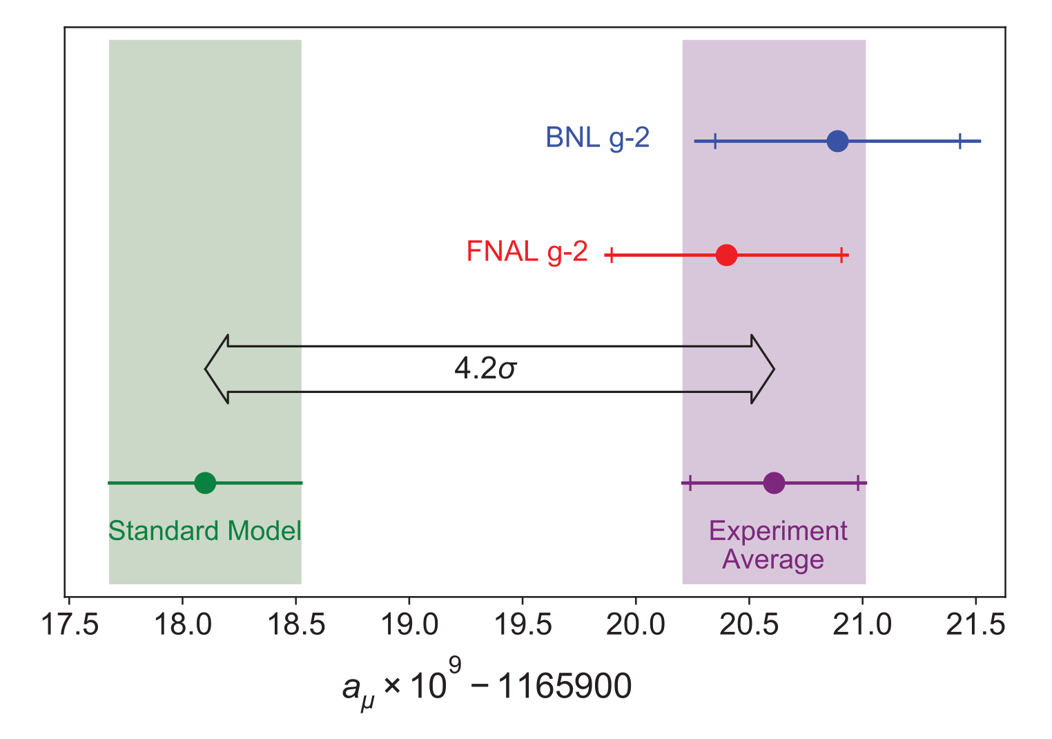


 , which is given by
 .
. ). At the same time, if the muons are polarized, meaning that their spin vector points along a particular direction when first injected into the storage ring, then this spin vector will also rotate when subjected to a uniform magnetic field. The frequency of the spin vector rotation is called the spin frequency (symbol
  ).
).
 is the muon mass,
  is the muon charge, and
  is the (ideally) uniform magnetic field. Once the precession frequency and the exact magnetic field are measured, one can immediately invert this equation to obtain
  is to rewrite the equation above into more experimentally amenable quantities:
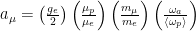
 is the proton-to-electron magnetic moment ratio,
  is the electon g-factor, and
  is the free proton’s Larmor frequency averaged over the muon beam spatial transverse distribution. The Larmor frequency measures the proton’s magnetic moment precession about the magnetic field and is directly proportional to B. The
  ). Recalling that the final desired accuracy for the left-hand side of the equation above is 140 ppb leads to a budget of 70 ppb for each of the
  measurements. This is perhaps a good point to stop and appreciate just how small these uncertainty budgets are: 1 ppb is a 1/1000000000 level of accuracy!


![N(t) = N_0 \; e^{-t/\tau} \left[ 1 + A_0 \; \text{cos}(\omega_a t + \phi_0) \right]](https://s0.wp.com/latex.php?latex=N%28t%29+%3D+N_0+%5C%3B+e%5E%7B-t%2F%5Ctau%7D+%5Cleft%5B+1+%2B+A_0+%5C%3B+%5Ctext%7Bcos%7D%28%5Comega_a+t+%2B+%5Cphi_0%29+%5Cright%5D+&bg=ffffff&fg=000&s=0&c=20201002)
 , the initial number of positrons;
  , the time-dilated muon lifetime;
  , the amplitude of the oscillation which is related to the asymmetry in the positron’s transverse impact position;
  , the phase of the oscillation.
 , and the two are related by:
![\omega_a(R) = 2 \pi \left(0.2291 \text{MHz} \right) \left[ 1 + (R + \Delta R) / 10^6 \right]](https://s0.wp.com/latex.php?latex=%5Comega_a%28R%29+%3D+2+%5Cpi+%5Cleft%280.2291+%5Ctext%7BMHz%7D+%5Cright%29+%5Cleft%5B+1+%2B+%28R+%2B+%5CDelta+R%29+%2F+10%5E6+%5Cright%5D+&bg=ffffff&fg=000&s=0&c=20201002) .
. is an arbitrary offset that is independently chosen by each different analysis group. This ensures that results from one group do not influence the others and allows all analysis to have the same (unknown) reference. We can expect a similar analysis (and probably several different types of
 and a
and a  boson, which is one of the three bosons that mediates weak force interactions. Then, the
  and electron neutrino
  . However, we can’t “stop” this process and observe the
  , which describes the strength of a magnetic source. This relationship for the muon can be expressed mathematically as
  ,
, gives the particle’s spin, e is the charge of an electron, and
  is the muon’s mass.
  , we further parametrize this difference by defining the anomalous magnetic dipole moment directly as
  .
.  , Z, and Higgs boson interactions) and the hadronic sector (quark and gluon interactions). We can explicitly split up the SM value of
  according to each of these contributions,
 .
.
 , 2) two muons and a
  boson, 3) two W bosons and a neutrino
  , and 4) two muons and a photon
  , while the SM makes a prediction of
  (both come with various error bars on the last 1-2 digits). Although they seem close, they differ by a factor of 3.7
 . HVP is the hadronic vacuum polarization (a process in which the virtual photon loop contains a quark-antiquark pair), while HLbL is hadronic light by light scattering (a process that is similar but involves more virtual photons). These two are main source of uncertainty in the SM theory prediction. Source: Muon g-2 Theory Initiative.


