Demonstration of probability density function as the output of a neural network. (Source: paper)
The simulation of particle collisions at the LHC is a pharaonic task. The messy chromodynamics of protons must be modeled; the statistics of the collision products must reflect the Standard Model; each particle has to travel through the detectors and interact with all the elements in its path. Its presence will eventually be reduced to electronic measurements, which, after all, is all we know about it.
The work of the simulation ends somewhere here, and that of the reconstruction starts; namely to go from electronic signals to particles. Reconstruction is a process common to simulation and to the real world. Starting from the tangle of statistical and detector effects that the actual measurements include, the goal is to divine the properties of the initial collision products.
Now, researchers at the Argonne National Laboratory looked into going from the simulated particles as produced in the collisions (aka “truth objects”) directly to the reconstructed ones (aka “reco objects”): bypassing the steps of the detailed interaction with the detectors and of the reconstruction algorithm could make the studies that use simulations much more speedy and efficient.
Display of a collision event involving hadronic jets at ATLAS. Each colored block corresponds to interaction with a detector element. (Source: ATLAS experiment)
The team used a neural network which it trained on simulations of the full set. The goal was to have the network learn to produce the properties of the reco objects when given only the truth objects. The process succeeded in producing the transverse momenta of hadronic jets, and looks suitable for any kind of particle and for other kinematic quantities.
More specifically, the researchers began with two million simulated jet events, fully passed through the ATLAS experiment and the reconstruction algorithm. For each of them, the network took the kinematic properties of the truth jet as input and was trained to achieve the reconstructed transverse momentum.
The network was taught to perform multi-categorization: its output didn’t consist of a single node giving the momentum value, but of 400 nodes, each corresponding to a different range of values. The output of each node was the probability for that particular range. In other words, the result was a probability density function for the reconstructed momentum of a given jet.
The final step was to select the momentum randomly from this distribution. For half a million of test jets, all this resulted in good agreement with the actual reconstructed momenta, specifically within 5% for values above 20 GeV. In addition, it seems that the training was sensitive to the effects of quantities other than the target one (e.g. the effects of the position in the detector), as the neural network was able to pick up on the dependencies between the input variables. Also, hadronic jets are complicated animals, so it is expected that the method will work on other objects just as well.
Comparison of the reconstructed transverse momentum between the full simulation and reconstruction (“Delphes”) and the neural net output. (Source: paper)
All in all, this work showed the perspective for neural networks to imitate successfully the effects of the detector and the reconstruction. Simulations in large experiments typically take up loads of time and resources due to their size, intricacy and frequent need for updates in the hardware conditions. Such a shortcut, needing only small numbers of fully processed events, would speed up studies such as optimization of the reconstruction and detector upgrades.
The landscape of direct detection of dark matter is a perplexing one; all experiments have so far come up with deafening silence, except for a single one which promises a symphony. This is the DAMA/LIBRA experiment in Gran Sasso, Italy, which has been seeing an annual modulation in its signal for two decades now.
Such an annual modulation is as dark-matter-like as it gets. First proposed by Katherine Freese in 1987, it would be the result of earth’s motion inside the galactic halo of dark matter in the same direction as the sun for half of the year and in the opposite direction during the other half. However, DAMA/LIBRA’s results are in conflict with other experiments – but with the catch that none of those used the same setup. The way to settle this is obviously to build more experiments with the DAMA/LIBRA setup. This is an ongoing effort which ultimately focuses on the crystals at its heart.
Cylindrical crystals wrapped in reflector, bounded by photomultipliers (PMTs) and surrounded by scintillators. (COSINE-100)
The specific crystals are made of the scintillating material thallium-doped sodium iodide, NaI(Tl). Dark matter particles, and particularly WIMPs, would collide elastically with atomic nuclei and the recoil would give off photons, which would eventually be captured by photomultiplier tubes at the ends of each crystal.
Right now a number of NaI(Tl)-based experiments are at various stages of preparation around the world, with COSINE-100 at the Yangyang mountain, S.Korea, already producing negative results. However, these are still not on equal footing with DAMA/LIBRA’s because of higher backgrounds at COSINE-100. What is the collaboration to do, then? The answer is focus even more on the crystals and how they are prepared.
Over the last couple of years some serious R&D went into growing better crystals for COSINE-200, the planned upgrade of COSINE-100. Yes, a crystal is something that can and does grow. A seed placed inside the raw material, in this case NaI(Tl) powder, leads it to organize itself around the seed’s structure over the next hours ordays.
In COSINE-100 the most annoying backgrounds came from within the crystals themselves because of the production process, because of natural radioactivity, and because of cosmogenically induced isotopes. Let’s see how each of these was tackled during the experiment’s mission towards a radiopure upgrade.
Improved techniques of growing and preparing the crystals reduced contamination from the materials of the grower device and from the ambient environment. At the same time different raw materials were tried out to put the inherent contamination under control.
Among a handful of naturally present radioactive isotopes particular care was given to 40K. 40K can decay characteristically to an X-ray of 3.2keV and a γ-ray of 1,460keV, a combination convenient for tagging it to a large extent. The tagging is done with the help of 2,000 liters of liquid scintillator surrounding the crystals. However, if the γ-ray escapes the crystal then the left-behind X-ray will mimic the expected signal from WIMPs… Eventually the dangerous 40K was brought down to levels comparable to those in DAMA/LIBRA through the investigation of various techniques and first materials.
But the main source of radioactive background in COSINE-100 was isotopes such as 3H or 22Na created inside the crystalsby cosmic ray muons,after their production. Now, their abundance was reduced significantly by two simple moves: the crystals were grown locally at a very low altitude and installed underground within a few weeks (instead of being transported from a lab at 1,400 meters above sea in Colorado). Moreover, most of the remaining cosmogenic background is to decay away within a couple of years.
Components of the background, and temporal evolution of the cosmogenic radioactivity. (Source)
Where are these efforts standing? The energy range of interest for testing the DAMA/LIBRA signal is 1-6keV. This corresponds to a background target of 1 count/kg/day/keV. After the crystals R&D, the achieved contamination was less than about 0.34 counts. In short, everything is ready for COSINE-100 to upgrade to COSINE-200 and test the annual modulation without the previous ambiguities that stood in the way.
If dark matter actually consists of a new kind of particle, then the most up-and-coming candidate is the axion. The axion is a consequence of the Peccei-Quinn mechanism, a plausible solution to the “strong CP problem,” or why the strong nuclear force conserves the CP-symmetry although there are no reasons for it to. It is a very light neutral boson, named by Frank Wilczek after a detergent brand (in a move that obviously dates its introduction in the ’70s).
Axion decay in a magnetic field: the result is a photon. (Source.)
Most experiments that try to directly detect dark matter have looked for WIMPs (weakly interacting massive particles). However, as those searches have not borne fruit, the focus started turning to axions, which make for good candidates given their properties and the fact that if they exist, then they exist in multitudes throughout the galaxies. Axions “speak” to the QCD part of the Standard Model, so they can appear in interaction vertices with hadronic loops. The end result is that axions passing through a magnetic field will convert to photons.
In practical terms, their detection boils down to having strong magnets, sensitive electronics and an electromagnetically very quiet place at one’s disposal. One can then sit back and wait for the hypothesized axions to pass through the detector as earth moves through the dark matter halo surrounding the Milky Way. Which is precisely why such experiments are known as “haloscopes.”
Now, the most veteran haloscope of all published significant new results. Alas, it is still empty-handed, but we can look at why its update is important and how it was reached.
ADMX (Axion Dark Matter eXperiment) of the University of Washington has been around for a quarter-century. By listening for signals from axions, it progressively gnaws away at the space of allowed values for their mass and coupling to photons, focusing on an area of interest:
Latest exclusion limits on the axion mass and coupling to photons.
Unlike higher values, this area is not excluded by astrophysical considerations (e.g. stars cooling off through axion emission) and other types of experiments (such as looking for axions from the sun). In addition, the bands above the lines denoted “KSVZ” and “DFSZ” are special. They correspond to the predictions of two models with favorable theoretical properties. So, ADMX is dedicated to scanning this parameter space. And the new analysis added one more year of data-taking, making a significant dent in this ballpark.
As mentioned, the presence of axions would be inferred from a stream of photons in the detector. The excluded mass range was scanned by “tuning” the experiment to different frequencies, while at each frequency step longer observation times probed smaller values for the axion-photon coupling.
Two things that this search needs is a lot of quiet and some good amplification, as the signal from a typical axion is expected to be as weak as the signal from a mobile phone left on the surface of Mars (around 10-23W). The setup is indeed stripped of noise by being placed in a dilution refrigerator, which keeps its temperature at a few tenths of a degree above absolute zero. This is practically the domain governed by quantum noise, so advantage can be taken of the finesse of quantum technology: for the first time ADMX used SQUIDs, superconducting quantum interference devices, for the amplification of the signal.
The heart of the experiment inside the refrigerator. The resonant frequency of the cavity is tuned to match the photons -hopefully- given off by axions. (Source.)
In the end, a good chunk of the parameter space which is favored by the theory might have been excluded, but the haloscope is ready to look at the rest of it. Just think of how, one day, a pulse inside a small device in a university lab might be a messenger of the mysteries unfolding across the cosmos.
Collisions at the Large Hadron Collider happen fast. 40 million times a second, bunches of 1011 protons are smashed together. The rate of these collisions is so fast that the computing infrastructure of the experiments can’t keep up with all of them. We are not able to read out and store the result of every collision that happens, so we have to ‘throw out’ nearly all of them. Luckily most of these collisions are not very interesting anyways. Most of them are low energy interactions of quarks and gluons via the strong force that have been already been studied at previous colliders. In fact, the interesting processes, like ones that create a Higgs boson, can happen billions of times less often than the uninteresting ones.
A plot showing the rates of different processes that can happen in a proton-proton collider like the LHC. We can see that the processes that are the most interesting, like the ones involving the Higgs boson (H), happen many orders of magnitude less often than the common ones.
The LHC experiments are thus faced with a very interesting challenge, how do you decide extremely quickly whether an event is interesting and worth keeping or not? This what the ‘trigger’ system, the Marie Kondo of LHC experiments, are designed to do. CMS for example has a two-tiered trigger system. The first level has 4 microseconds to make a decision and must reduce the event rate from 40 millions events per second to 100,000. This speed requirement means the decision has to be made using at the hardware level, requiring the use of specialized electronics to quickly to synthesize the raw information from the detector into a rough idea of what happened in the event. Selected events are then passed to the High Level Trigger (HLT), which has 150 milliseconds to run versions of the CMS reconstruction algorithms to further reduce the event rate to a thousand per second.
While this system works very well for most uses of the data, like measuring the decay of Higgs bosons, sometimes it can be a significant obstacle. If you want to look through the data for evidence of a new particle that is relatively light, it can be difficult to prevent the trigger from throwing out possible signal events. This is because one of the most basic criteria the trigger uses to select ‘interesting’ events is that they leave a significant amount of energy in the detector. But the decay products of a new particle that is relatively light won’t have a substantial amount of energy and thus may look ‘uninteresting’ to the trigger.
In order to get the most out of their collisions, experimenters are thinking hard about these problems and devising new ways to look for signals the triggers might be missing. One idea is to save additional events from the HLT in a substantially reduced size. Rather than saving the raw information from the event, that can be fully processed at a later time, instead the only the output of the quick reconstruction done by the trigger is saved. At the cost of some precision, this can reduce the size of each event by roughly two orders of magnitude, allowing events with significantly lower energy to be stored. CMS and ATLAS have used this technique to look for new particles decaying to two jets and LHCb has used it to look for dark photons. The use of these fast reconstruction techniques allows them to search for, and rule out the existence of, particles with much lower masses than otherwise possible. As experiments explore new computing infrastructures (like GPU’s) to speed up their high level triggers, they may try to do even more sophisticated analyses using these techniques.
CMS’s limits on the existence of a new particle decaying to two jets. The search in the ‘low mass’ region is only possible due to the use of saving the fast reconstruction of the trigger. (source)
But experimenters aren’t just satisfied with getting more out of their high level triggers, they want to revamp the low-level ones as well. In order to get these hardware-level triggers to make smarter decisions, experimenters are trying get them to run machine learning models. Machine learning has become very popular tool to look for rare signals in LHC data. One of the advantages of machine learning models is that once they have been trained, they can make complex inferences in a very short amount of time. Perfect for a trigger! Now a group of experimentalists have developed a library that can translate the most popular types machine learning models into a format that can be run on the Field Programmable Gate Arrays used in lowest level triggers. This would allow experiments to quickly identify events from rare signals that have complex signatures that the current low-level triggers don’t have time to look for.
The LHC experiments are working hard to get the most out their collisions. There could be particles being produced in LHC collisions already but we haven’t been able to see them because of our current triggers, but these new techniques are trying to cover our current blind spots. Look out for new ideas on how to quickly search for interesting signatures, especially as we get closer the high luminosity upgrade of the LHC.
Article: “Anomaly Detection for Resonant New Physics with Machine Learning”
Authors: Jack H. Collins, Kiel Howe, Benjamin Nachman
Reference : https://arxiv.org/abs/1805.02664
One of the main goals of LHC experiments is to look for signals of physics beyond the Standard Model; new particles that may explain some of the mysteries the Standard Model doesn’t answer. The typical way this works is that theorists come up with a new particle that would solve some mystery and they spell out how it interacts with the particles we already know about. Then experimentalists design a strategy of how to search for evidence of that particle in the mountains of data that the LHC produces. So far none of the searches performed in this way have seen any definitive evidence of new particles, leading experimentalists to rule out a lot of the parameter space of theorists favorite models.
A summary of searches the ATLAS collaboration has performed. The left columns show model being searched for, what experimental signature was looked at and how much data has been analyzed so far. The color bars show the regions that have been ruled out based on the null result of the search. As you can see, we have already covered a lot of territory.
Despite this extensive program of searches, one might wonder if we are still missing something. What if there was a new particle in the data, waiting to be discovered, but theorists haven’t thought of it yet so it hasn’t been looked for? This gives experimentalists a very interesting challenge, how do you look for something new, when you don’t know what you are looking for? One approach, which Particle Bites has talked about before, is to look at as many final states as possible and compare what you see in data to simulation and look for any large deviations. This is a good approach, but may be limited in its sensitivity to small signals. When a normal search for a specific model is performed one usually makes a series of selection requirements on the data, that are chosen to remove background events and keep signal events. Nowadays, these selection requirements are getting more complex, often using neural networks, a common type of machine learning model, trained to discriminate signal versus background. Without some sort of selection like this you may miss a smaller signal within the large amount of background events.
This new approach lets the neural network itself decide what signal to look for. It uses part of the data itself to train a neural network to find a signal, and then uses the rest of the data to actually look for that signal. This lets you search for many different kinds of models at the same time!
If that sounds like magic, lets try to break it down. You have to assume something about the new particle you are looking for, and the technique here assumes it forms a resonant peak. This is a common assumption of searches. If a new particle were being produced in LHC collisions and then decaying, then you would get an excess of events where the invariant mass of its decay products have a particular value. So if you plotted the number of events in bins of invariant mass you would expect a new particle to show up as a nice peak on top of a relatively smooth background distribution. This is a very common search strategy, and often colloquially referred to as a ‘bump hunt’. This strategy was how the Higgs boson was discovered in 2012.
A histogram showing the invariant mass of photon pairs. The Higgs boson shows up as a bump at 125 GeV. Plot from here
The other secret ingredient we need is the idea of Classification Without Labels (abbreviated CWoLa, pronounced like koala). The way neural networks are usually trained in high energy physics is using fully labeled simulated examples. The network is shown a set of examples and then guesses which are signal and which are background. Using the true label of the event, the network is told which of the examples it got wrong, its parameters are updated accordingly, and it slowly improves. The crucial challenge when trying to train using real data is that we don’t know the true label of any of data, so its hard to tell the network how to improve. Rather than trying to use the true labels of any of the events, the CWoLA technique uses mixtures of events. Lets say you have 2 mixed samples of events, sample A and sample B, but you know that sample A has more signal events in it than sample B. Then, instead of trying to classify signal versus background directly, you can train a classifier to distinguish between events from sample A and events from sample B and what that network will learn to do is distinguish between signal and background. You can actually show that the optimal classifier for distinguishing the two mixed samples is the same as the optimal classifier of signal versus background. Even more amazing, this technique actually works quite well in practice, achieving good results even when there is only a few percent of signal in one of the samples.
An illustration of the CWoLa method. A classifier trained to distinguish between two mixed samples of signal and background events learns can learn to classify signal versus background. Taken from here
The technique described in the paper combines these two ideas in a clever way. Because we expect the new particle to show up in a narrow region of invariant mass, you can use some of your data to train a classifier to distinguish between events in a given slice of invariant mass from other events. If there is no signal with a mass in that region then the classifier should essentially learn nothing, but if there was a signal in that region that the classifier should learn to separate signal and background. Then one can apply that classifier to select events in the rest of your data (which hasn’t been used in the training) and look for a peak that would indicate a new particle. Because you don’t know ahead of time what mass any new particle should have, you scan over the whole range you have sufficient data for, looking for a new particle in each slice.
The specific case that they use to demonstrate the power of this technique is for new particles decaying to pairs of jets. On the surface, jets, the large sprays of particles produced when quark or gluon is made in a LHC collision, all look the same. But actually the insides of jets, their sub-structure, can contain very useful information about what kind of particle produced it. If a new particle that is produced decays into other particles, like top quarks, W bosons or some a new BSM particle, before decaying into quarks then there will be a lot of interesting sub-structure to the resulting jet, which can be used to distinguish it from regular jets. In this paper the neural network uses information about the sub-structure for both of the jets in event to determine if the event is signal-like or background-like.
The authors test out their new technique on a simulated dataset, containing some events where a new particle is produced and a large number of QCD background events. They train a neural network to distinguish events in a window of invariant mass of the jet pair from other events. With no selection applied there is no visible bump in the dijet invariant mass spectrum. With their technique they are able to train a classifier that can reject enough background such that a clear mass peak of the new particle shows up. This shows that you can find a new particle without relying on searching for a particular model, allowing you to be sensitive to particles overlooked by existing searches.
Demonstration of the bump hunt search. The shaded histogram is the amount of signal in the dataset. The different levels of blue points show the data remaining after applying tighter and tighter selection based on the neural network classifier score. The red line is the predicted amount of background events based on fitting the sideband regions. One can see that for the tightest selection (bottom set of points), the data forms a clear bump over the background estimate, indicating the presence of a new particle
This paper was one of the first to really demonstrate the power of machine-learning based searches. There is actually a competition being held to inspire researchers to try out other techniques on a mock dataset. So expect to see more new search strategies utilizing machine learning being released soon. Of course the real excitement will be when a search like this is applied to real data and we can see if machines can find new physics that us humans have overlooked!
Read More:
Quanta Magazine Article “How Artificial Intelligence Can Supercharge the Search for New Particles”
Blog Post on the CWoLa Method “Training Collider Classifiers on Real Data”
Particle Bites Post “Going Rogue: The Search for Anything (and Everything) with ATLAS”
Blog Post on applying ML to top quark decays “What does Bidirectional LSTM Neural Networks has to do with Top Quarks?”
When theorists were first developing quantum field theory in the 1940’s they quickly ran into a problem. Some of their calculations kept producing infinities which didn’t make physical sense. After scratching their heads for a while they eventually came up with a procedure known as renormalization to solve the problem. Renormalization neatly hid away the infinities that were plaguing their calculations by absorbing them into the constants (like masses and couplings) in the theory, but it also produced some surprising predictions. Renormalization said that all these ‘constants’ weren’t actually constant at all! The value of these ‘constants’ depended on the energy scale at which you probed the theory.
One of the most famous realizations of this phenomena is the ‘running’ of the strong coupling constant. The value of a coupling encodes the strength of a force. The strong nuclear force, responsible for holding protons and neutrons together, is actually so strong at low energies our normal techniques for calculation don’t work. But in 1973, Gross, Wilczek and Politzer realized that in quantum chromodynamics (QCD), the quantum field theory describing the strong force, renormalization would make the strong coupling constant ‘run’ smaller at high energies. This meant at higher energies one could use normal perturbative techniques to do calculations. This behavior of the strong force is called ‘asymptotic freedom’ and earned them a Nobel prize. Thanks to asymptotic freedom, it is actually much easier for us to understand what QCD predicts for high energy LHC collisions than for the properties of bound states like the proton.
Figure 1: The value of the strong coupling constant (α_s) is plotted as a function of the energy scale. Data from multiple experiments at different energies are compared to the prediction from QCD of how it should run. From [5]Now for the first time, CMS has measured the running of a new fundamental parameter, the mass of the top quark. More than just being a cool thing to see, measuring how the top quark mass runs tests our understanding of QCD and can also be sensitive to physics beyond the Standard Model. The top quark is the heaviest fundamental particle we know about, and many think that it has a key role to play in solving some puzzles of the Standard Model. In order to measure the top quark mass at different energies, CMS used the fact that the rate of producing a top quark-antiquark pair depends on the mass of the top quark. So by measuring this rate at different energies they can extract the top quark mass at different scales.
Top quarks nearly always decay into W-bosons and b quarks. Like all quarks, the b quarks then create a large shower of particles before they reach the detector called a jet. The W-bosons can decay either into a lepton and a neutrino or two quarks. The CMS detector is very good at reconstructing leptons and jets, but neutrinos escape undetected. However one can infer the presence of neutrinos in an event because we know energy must be conserved in the collision, so if neutrinos are produced we will see ‘missing’ energy in the event. The CMS analyzers looked for top anti-top pairs where one W-boson decayed to an electron and a neutrino and the other decayed to a muon and a neutrino. By using information about the electron, muon, missing energy, and jets in an event, the kinematics of the top and anti-top pair can be reconstructed.
The measured running of the top quark mass is shown in Figure 2. The data agree with the predicted running from QCD at the level of 1.1 sigma, and the no-running hypothesis is excluded at above 95% confidence level. Rather than being limited by the amount of data, the main uncertainties in this result come from the theoretical understanding of the top quark production and decay, which the analyzers need to model very precisely in order to extract the top quark mass. So CMS will need some help from theorists if they want to improve this result in the future.
Figure 2: The ratio of the top quark mass compared to its mass at a reference scale (476 GeV) is plotted as a function of energy. The red line is the theoretical prediction of how the mass should run in QCD.
When a single experimental collaboration has a few thousand contributors (and even more opinions), there are a lot of rules. These rules dictate everything from how you get authorship rights to how you get chosen to give a conference talk. In fact, this rulebook is so thorough that it could be the topic of a whole other post. But for now, I want to focus on one rule in particular, a rule that has only been around for a few decades in particle physics but is considered one of the most important practices of good science: blinding.
In brief, blinding is the notion that it’s experimentally compromising for a scientist to look at the data before finalizing the analysis. As much as we like to think of ourselves as perfectly objective observers, the truth is, when we really really want a particular result (let’s say a SUSY discovery), that desire can bias our work. For instance, imagine you were looking at actual collision data while you were designing a signal region. You might unconsciously craft your selection in such a way to force an excess of data over background prediction. To avoid such human influences, particle physics experiments “blind” their analyses while they are under construction, and only look at the data once everything else is in place and validated.
Figure 1: “Blind analysis: Hide results to seek the truth”, R. MacCounor & S. Perlmutter for Nature.com
This technique has kept the field of particle physics in rigorous shape for quite a while. But there’s always been a subtle downside to this practice. If we only ever look at the data after we finalize an analysis, we are trapped within the confines of theoretically motivated signatures. In this blinding paradigm, we’ll look at all the places that theory has shone a spotlight on, but we won’t look everywhere. Our whole game is to search for new physics. But what if amongst all our signal regions and hypothesis testing and neural net classifications… we’ve simply missed something?
It is this nagging question that motivates a specific method of combing the LHC datasets for new physics, one that the authors of this paper call a “structured, global and automated way to search for new physics.” With this proposal, we can let the data itself tell us where to look and throw unblinding caution to the winds.
The idea is simple: scan the whole ATLAS dataset for discrepancies, setting a threshold for what defines a feature as “interesting”. If this preliminary scan stumbles upon a mysterious excess of data over Standard Model background, don’t just run straight to Stockholm proclaiming a discovery. Instead, simply remember to look at this area again once more data is collected. If your feature of interest is a fluctuation, it will wash out and go away. If not, you can keep watching it until you collect enough statistics to do the running to Stockholm bit. Essentially, you let a first scan of the data rather than theory define your signal regions of interest. In fact, all the cool kids are doing it: H1, CDF, D0, and evenATLASandCMS have performed earlier versions of this general search.
The nuts and bolts of this particular paper include 3.2 fb-1 of 2015 13 TeV LHC data to try out. Since the whole goal of this strategy is to be as general as possible, we might as well go big or go home with potential topologies. To that end, the authors comb through all the data and select any event “involving high pT isolated leptons (electrons and muons), photons, jets, b-tagged jets and missing transverse momentum”. All of the backgrounds are simply modeled with Monte Carlo simulation.
Once we have all these events, we need to sort them. Here, “the classification includes all possible final state configurations and object multiplicities, e.g. if a data event with seven reconstructed muons is found it is classified in a ‘7- muon’ event class (7μ).” When you add up all the possible permutations of objects and multiplicities, you come up with a cool 639 event classes with at least 1 data event and a Standard Model expectation of at least 0.1.
From here, it’s just a matter of checking data vs. MC agreement and the pulls for each event class. The authors also apply some measures to weed out the low stat or otherwise sketchy regions; for instance, 1 electron + many jets is more likely to be multijet faking a lepton and shouldn’t necessarily be considered as a good event category. Once this logic applied, you can plot all of your SRs together grouped by category; Figure 2 shows an example for the multijet events. The paper includes 10 of these plots in total, with regions ranging in complexity from nothing but 1μ1j to more complicated final states like ETmiss2μ1γ4j (say that five times fast.)
Figure 2: The number of events in data and for the different SM background predictions considered. The classes are labeled according to the multiplicity and type (e, μ, γ, j, b, ETmiss) of the reconstructed objects for this event class. The hatched bands indicate the total uncertainty of the SM prediction.
Once we can see data next to Standard Model prediction for all these categories, it’s necessary to have a way to measure just how unusual an excess may be. The authors of this paper implement an algorithm that searches for the region of largest deviation in the distributions of two variables that are good at discriminating background from new physics. These are the effective mass, the sum of all jet and missing momenta, and the invariant mass, computed with all visible objects and no missing energy.
For each deviation found, a simple likelihood function is built as the convolution of probability density functions (pdfs): one Poissonian pdf to describe the event yields, and Gaussian pdfs for each systematic uncertainty. The integral of this function, p0, is the probability that the Standard Model expectation fluctuated to the observed yield. This p0 value is an industry standard in particle physics: a value of p0 < 3e-7 is our threshold for discovery.
Sadly (or reassuringly), the smallest p0 value found in this scan is 3e-04 (in the 1m1e4b2j event class). To figure out precisely how significant this value is, the authors ran a series of pseudoexperiments for each event class and applied the same scanning algorithm to them, to determine how often such a deviation would occur in a wholly different fake dataset. In fact, a p0 of 3e-04 was expected 70% of the pseudoexperiments.
So the excesses that were observed are not (so far) significant enough to focus on. But the beauty of this analysis strategy is that this deviation can be easily followed up with the addition of a newer dataset. Think of these general searches as the sidekick of the superheros that are our flagship SUSY, exotics, and dark matter searches. They can help us dot i’s and cross t’s, make sure nothing falls through the cracks— and eventually, just maybe, make a discovery.
March is an exciting month for high energy physicists. Every year at this time, scientists from all over the world gather for the annual Moriond Conference, where all of the latest results are shown and discussed. Now that this physics Christmas season is over, I, like many other physicists, am sifting through the proceedings, trying to get a hint of what is the new cool physics to be chasing after. My conclusions? The Higgsino search is high on this list.
Physicists chatting at the 2017 Moriond Conference. Image credit ATLAS-PHOTO-2017-009-1.
The search for Higgsinos falls under the broad and complex umbrella of searches for supersymmetry (SUSY). We’ve talked about SUSY on Particlebites in the past; see a recent post on thestop search for reference. Recall that the basic prediction of SUSY is that every boson in the Standard Model has a fermionic supersymmetric partner, and every fermion gets a bosonic partner.
So then what exactly is a Higgsino? The naming convention of SUSY would indicate that the –ino suffix means that a Higgsino is the supersymmetric partner of the Higgs boson. This is partly true, but the whole story is a bit more complicated, and requires some understanding of the Higgs mechanism.
To summarize, in our Standard Model, the photon carries the electromagnetic force, and the W and Z carry the weak force. But before electroweak symmetry breaking, these bosons did not have such distinct tasks. Rather, there were three massless bosons, the B, W, and Higgs, which together all carried the electroweak force. It is the supersymmetric partners of these three bosons that mix to form new mass eigenstates, which we call simply charginos or neutralinos, depending on their charge. When we search for new particles, we are searching for these mass eigenstates, and then interpreting our results in the context of electroweak-inos.
SUSY searches can be broken into many different analyses, each targeting a particular particle or group of particles in this new sector. Starting with the particles that are suspected to have low mass is a good idea, since we’re more likely to observe these at the current LHC collision energy. If we begin with these light particles, and add in the popular theory of naturalness, we conclude that Higgsinos will be the easiest to find of all the new SUSY particles. More specifically, the theory predicts three Higgsinos that mix into two neutralinos and a chargino, each with a mass around 200-300 GeV, but with a very small mass splitting between the three. See Figure 1 for a sample mass spectra of all these particles, where N and C indicate neutralino or chargino respectively (keep in mind this is just a possibility; in principle, any bino/wino/higgsino mass hierarchy is allowed.)
Figure 1: Sample electroweak SUSY mass spectrum. Image credit: T. Lari, INFN Milano
This is both good news and bad news. The good part is that we have reason to think that there are three Higgsinos with masses that are well within our reach at the LHC. The bad news is that this mass spectrum is very compressed, making the Higgsinos extremely difficult to detect experimentally. This is due to the fact that when C1 or N2 decays to N1 (the lightest neutralino), there is very little mass difference leftover to supply energy to the decay products. As a result, all of the final state objects (two N1s plus a W or a Z as a byproduct, see Figure 2) will have very low momentum and thus are very difficult to detect.
Figure 2: Electroweakino pair production and decay (CMS-PAS-SUS-16-048).
The CMS collaboration Higgsino analysis documented here uses a clever analysis strategy for such compressed decay scenarios. Since initial state radiation (ISR) jets occur often in proton-proton collisions, you can ask for your event to have one. This jet radiating from the collision will give the system a kick in the opposite direction, providing enough energy to those soft particles for them to be detectable. At the end of the day, the analysis team looks for events with ISR, missing transverse energy (MET), and two soft opposite sign leptons from the Z decay (to distinguish from hadronic SM-like backgrounds). Figure 3 shows a basic diagram of what these signal events would look like.
Figure 3: Signal event vector diagram. Image credit C. Botta, CERN
In order to conduct this search, several new analysis techniques were employed. Reconstruction of leptons at low pT becomes extremely important in this regime, and the standard cone isolation of the lepton and impact parameter cuts are used to ensure proper lepton identification. New discriminating variables are also added, which exploit kinematic information about the lepton and the soft particles around it, in order to distinguish “prompt” (signal) leptons from those that may have come from a jet and are thus “non prompt” (background.)
In addition, the analysis team paid special attention to the triggers that could be used to select signal events from the immense number of collisions, creating a new “compressed” trigger that uses combined information from both soft muons (pT > 5 GeV) and missing energy ( > 125 GeV).
With all of this effort, the group is able to probe down to a mass splitting between Higgsinos of 20 GeV, excluding N2 masses up to 230 GeV. This is an especially remarkable result because the current strongest limit on Higgsinos comes from the LEP experiment, a result that is over ten years old! Because the Higgsino searches are strongly limited by the low cross section of electroweak SUSY, additional data will certainly mean that these searches will proceed quickly, and more stringent bounds will be placed (or, perhaps, a discovery is in store!)
Figure 4: Figure 5: The observed exclusion contours (black) with the corresponding 1 standard deviation uncertainties. The dashed red curves present the expected limits with 1 SD experimental uncertainties (CMS-PAS-SUS-16-048).
Title: “Performance of algorithms that reconstruct missing transverse momentum in s = √8 TeV proton–proton collisions in the ATLAS detector” Authors: ATLAS Collaboration
Check out the public version of this post on the official ATLAS blog here!
The ATLAS experiment recently released a note detailing the nature and performance of algorithms designed to calculate what is perhaps the most difficult quantity in any LHC event: missing transverse energy. Missing energy is difficult because by its very nature, it is missing, thus making it unobservable in the detector. So where does this missing energy come from, and why do we even need it?
Figure 1
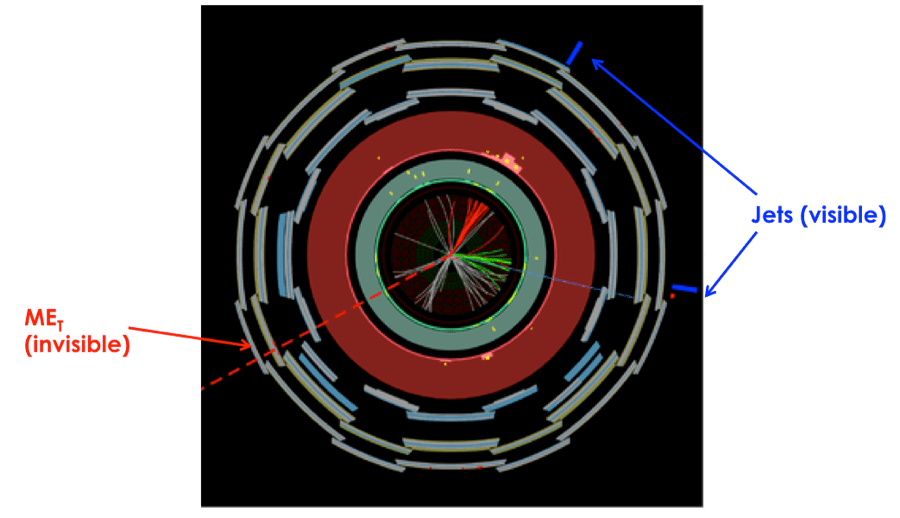
The LHC accelerate protons towards one another on the same axis, so they will collide head on. Therefore, the incoming partons have net momentum along the direction of the beamline, but no net momentum in the transverse direction (see Figure 1). MET is then defined as the negative vectorial sum (in the transverse plane) of all recorded particles. Any nonzero MET indicates a particle that escaped the detector. This escaping particle could be a regular Standard Model neutrino, or something much more exotic, such as the lightest supersymmetric particle or a dark matter candidate.
Figure 2
Figure 2 shows an event display where the calculated MET balances the visible objects in the detector. In this case, these visible objects are jets, but they could also be muons, photons, electrons, or taus. This constitutes the “hard term” in the MET calculation. Often there are also contributions of energy in the detector that are not associated to a particular physics object, but may still be necessary to get an accurate measurement of MET. This momenta is known as the “soft term”.
In the course of looking at all the energy in the detector for a given event, inevitably some pileup will sneak in. The pileup could be contributions from additional proton-proton collisions in the same bunch crossing, or from scattering of protons upstream of the interaction point. Either way, the MET reconstruction algorithms have to take this into account. Adding up energy from pileup could lead to more MET than was actually in the collision, which could mean the difference between an observation of dark matter and just another Standard Model event.
One of the ways to suppress pile up is to use a quantity called jet vertex fraction (JVF), which uses the additional information of tracks associated to jets. If the tracks do not point back to the initial hard scatter, they can be tagged as pileup and not included in the calculation. This is the idea behind the Track Soft Term (TST) algorithm. Another way to remove pileup is to estimate the average energy density in the detector due to pileup using event-by-event measurements, then subtracting this baseline energy. This is used in the Extrapolated Jet Area with Filter, or EJAF algorithm.
Once these algorithms are designed, they are tested in two different types of events. One of these is in W to lepton + neutrino decay signatures. These events should all have some amount of real missing energy from the neutrino, so they can easily reveal how well the reconstruction is working. The second group is Z boson to two lepton events. These events should not have any real missing energy (no neutrinos), so with these events, it is possible to see if and how the algorithm reconstructs fake missing energy. Fake MET often comes from miscalibration or mismeasurement of physics objects in the detector. Figures 3 and 4 show the calorimeter soft MET distributions in these two samples; here it is easy to see the shape difference between real and fake missing energy.
Figure 3: Distribution of the sum of missing energy in the calorimeter soft term shown in Z to μμ data and Monte Carlo events.
Figure 4: Distribution of the sum of missing energy in the calorimeter soft term shown in W to eν data and Monte Carlo events.
This note evaluates the performance of these algorithms in 8 TeV proton proton collision data collected in 2012. Perhaps the most important metric in MET reconstruction performance is the resolution, since this tells you how well you know your MET value. Intuitively, the resolution depends on detector resolution of the objects that went into the calculation, and because of pile up, it gets worse as the number of vertices gets larger. The resolution is technically defined as the RMS of the combined distribution of MET in the x and y directions, covering the full transverse plane of the detector. Figure 5 shows the resolution as a function of the number of vertices in Z to μμ data for several reconstruction algorithms. Here you can see that the TST algorithm has a very small dependence on the number of vertices, implying a good stability of the resolution with pileup.
Figure 5: Distribution of the sum of missing energy in the calorimeter soft term shown in W to eν data and Monte Carlo events.
Another important quantity to measure is the angular resolution, which is important in the reconstruction of kinematic variables such as the transverse mass of the W. It can be measured in W to μν simulation by comparing the direction of the MET, as reconstructed by the algorithm, to the direction of the true MET. The resolution is then defined as the RMS of the distribution of the phi difference between these two vectors. Figure 6 shows the angular resolution of the same five algorithms as a function of the true missing transverse energy. Note the feature between 40 and 60 GeV, where there is a transition region into events with high pT calibrated jets. Again, the TST algorithm has the best angular resolution for this topology across the entire range of true missing energy.
Figure 6: Resolution of ΔΦ(reco MET, true MET) for 0 jet W to μν Monte Carlo.
As the High Luminosity LHC looms larger and larger, the issue of MET reconstruction will become a hot topic in the ATLAS collaboration. In particular, the HLLHC will be a very high pile up environment, and many new pile up subtraction studies are underway. Additionally, there is no lack of exciting theories predicting new particles in Run 3 that are invisible to the detector. As long as these hypothetical invisible particles are being discussed, the MET teams will be working hard to catch them.
Article: Particle Physics Models for the 17 MeV Anomaly in Beryllium Nuclear Decays Authors: J.L. Feng, B. Fornal, I. Galon, S. Gardner, J. Smolinsky, T. M. P. Tait, F. Tanedo Reference:arXiv:1608.03591 (Submitted to Phys. Rev. D)
See also this Latin American Webinar on Physics recorded talk.
Also featuring the results from:
— Gulyás et al., “A pair spectrometer for measuring multipolarities of energetic nuclear transitions” (description of detector; 1504.00489; NIM)
— Krasznahorkay et al., “Observation of Anomalous Internal Pair Creation in 8Be: A Possible Indication of a Light, Neutral Boson” (experimental result; 1504.01527; PRL version; note PRL version differs from arXiv)
— Feng et al., “Protophobic Fifth-Force Interpretation of the Observed Anomaly in 8Be Nuclear Transitions” (phenomenology; 1604.07411; PRL)
Editor’s note: the author is a co-author of the paper being highlighted.
Recently there’s some press (see links below) regarding early hints of a new particle observed in a nuclear physics experiment. In this bite, we’ll summarize the result that has raised the eyebrows of some physicists, and the hackles of others.
A crash course on nuclear physics
Nuclei are bound states of protons and neutrons. They can have excited states analogous to the excited states of at lowoms, which are bound states of nuclei and electrons. The particular nucleus of interest is beryllium-8, which has four neutrons and four protons, which you may know from the triple alpha process. There are three nuclear states to be aware of: the ground state, the 18.15 MeV excited state, and the 17.64 MeV excited state.
Beryllium-8 excited nuclear states. The 18.15 MeV state (red) exhibits an anomaly. Both the 18.15 MeV and 17.64 states decay to the ground through a magnetic, p-wave transition. Image adapted from Savage et al. (1987).
Most of the time the excited states fall apart into a lithium-7 nucleus and a proton. But sometimes, these excited states decay into the beryllium-8 ground state by emitting a photon (γ-ray). Even more rarely, these states can decay to the ground state by emitting an electron–positron pair from a virtual photon: this is called internal pair creation and it is these events that exhibit an anomaly.
The beryllium-8 anomaly
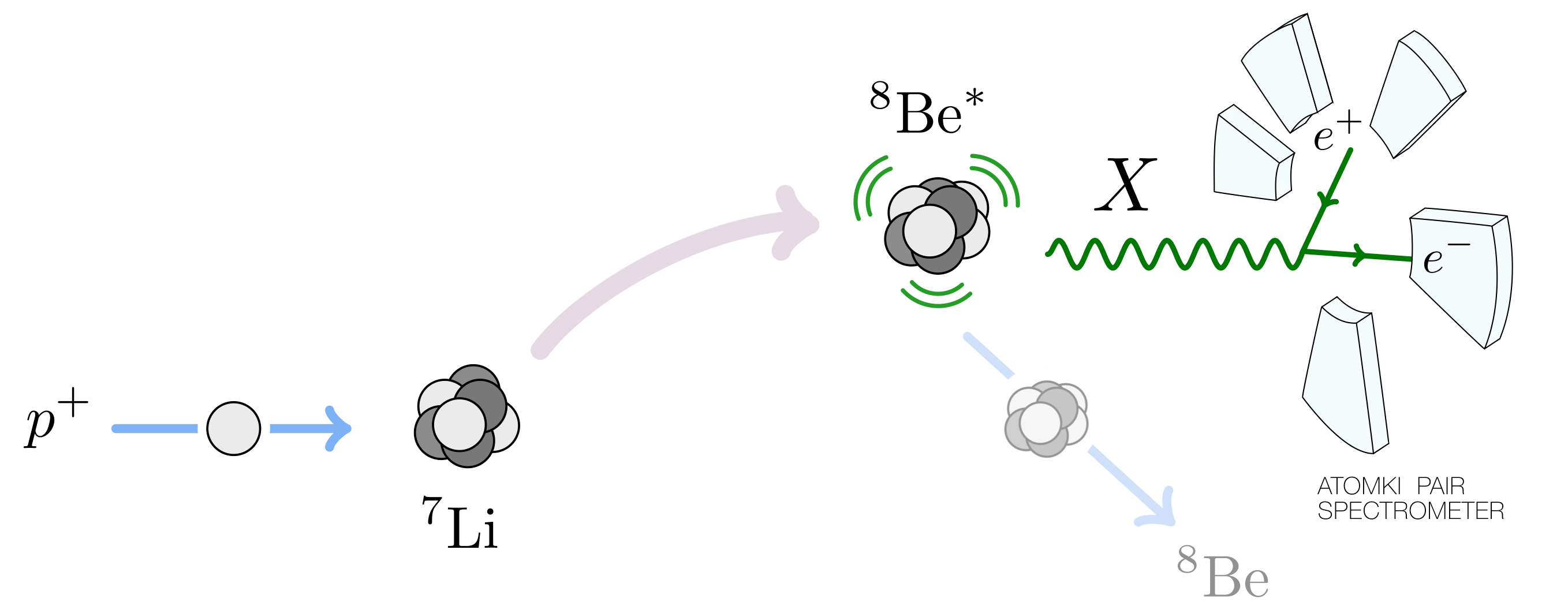
Physicists at the Atomki nuclear physics institute in Hungary were studying the nuclear decays of excited beryllium-8 nuclei. The team, led by Attila J. Krasznahorkay, produced beryllium excited states by bombarding a lithium-7 nucleus with protons.
Beryllium-8 excited states are prepare by bombarding lithium-7 with protons.
The proton beam is tuned to very specific energies so that one can ‘tickle’ specific beryllium excited states. When the protons have around 1.03 MeV of kinetic energy, they excite lithium into the 18.15 MeV beryllium state. This has two important features:
Picking the proton energy allows one to only produce a specific excited state so one doesn’t have to worry about contamination from decays of other excited states.
Because the 18.15 MeV beryllium nucleus is produced at resonance, one has a very high yield of these excited states. This is very good when looking for very rare decay processes like internal pair creation.
What one expects is that most of the electron–positron pairs have small opening angle with a smoothly decreasing number as with larger opening angles.
Expected distribution of opening angles for ordinary internal pair creation events. Each line corresponds to nuclear transition that is electric (E) or magenetic (M) with a given orbital quantum number, l. The beryllium transitionsthat we’re interested in are mostly M1. Adapted from Gulyás et al. (1504.00489).
Instead, the Atomki team found an excess of events with large electron–positron opening angle. In fact, even more intriguing: the excess occurs around a particular opening angle (140 degrees) and forms a bump.
Number of events (dN/dθ) for different electron–positron opening angles and plotted for different excitation energies (Ep). For Ep=1.10 MeV, there is a pronounced bump at 140 degrees which does not appear to be explainable from the ordinary internal pair conversion. This may be suggestive of a new particle. Adapted from Krasznahorkay et al., PRL 116, 042501.
Here’s why a bump is particularly interesting:
The distribution of ordinary internal pair creation events is smoothly decreasing and so this is very unlikely to produce a bump.
Bumps can be signs of new particles: if there is a new, light particle that can facilitate the decay, one would expect a bump at an opening angle that depends on the new particle mass.
Schematically, the new particle interpretation looks like this:
Schematic of the Atomki experiment and new particle (X) interpretation of the anomalous events. In summary: protons of a specific energy bombard stationary lithium-7 nuclei and excite them to the 18.15 MeV beryllium-8 state. These decay into the beryllium-8 ground state. Some of these decays are mediated by the new X particle, which then decays in to electron–positron pairs of a certain opening angle that are detected in the Atomki pair spectrometer detector. Image from 1608.03591.
As an exercise for those with a background in special relativity, one can use the relation to prove the result:
This relates the mass of the proposed new particle, X, to the opening angle θ and the energies E of the electron and positron. The opening angle bump would then be interpreted as a new particle with mass of roughly 17 MeV. To match the observed number of anomalous events, the rate at which the excited beryllium decays via the X boson must be 6×10⁻⁶ times the rate at which it goes into a γ-ray.
The anomaly has a significance of 6.8σ. This means that it’s highly unlikely to be a statistical fluctuation, as the 750 GeV diphoton bump appears to have been. Indeed, the conservative bet would be some not-understood systematic effect, akin to the 130 GeV Fermi γ-ray line.
The beryllium that cried wolf?
Some physicists are concerned that beryllium may be the ‘boy that cried wolf,’ and point to papers by the late Fokke de Boer as early as 1996 and all the way to 2001. de Boer made strong claims about evidence for a new 10 MeV particle in the internal pair creation decays of the 17.64 MeV beryllium-8 excited state. These claims didn’t pan out, and in fact the instrumentation paper by the Atomki experiment rules out that original anomaly.
The proposed evidence for “de Boeron” is shown below:
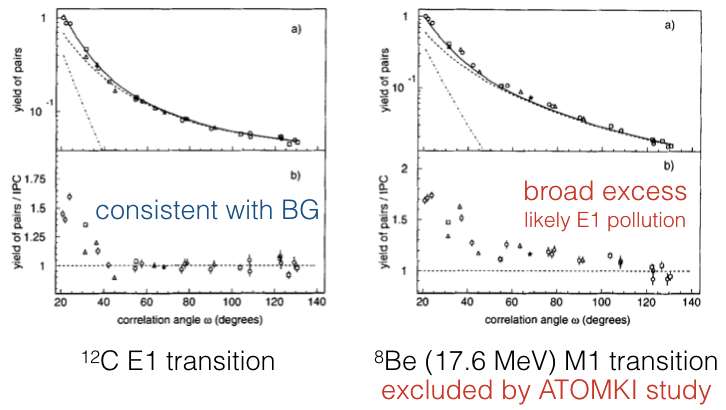
The de Boer claim for a 10 MeV new particle. Left: distribution of opening angles for internal pair creation events in an E1 transition of carbon-12. This transition has similar energy splitting to the beryllium-8 17.64 MeV transition and shows good agreement with the expectations; as shown by the flat “signal – background” on the bottom panel. Right: the same analysis for the M1 internal pair creation events from the 17.64 MeV beryllium-8 states. The “signal – background” now shows a broad excess across all opening angles. Adapted from de Boer et al. PLB 368, 235 (1996).
When the Atomki group studied the same 17.64 MeV transition, they found that a key background component—subdominant E1 decays from nearby excited states—dramatically improved the fit and were not included in the original de Boer analysis. This is the last nail in the coffin for the proposed 10 MeV “de Boeron.”
However, the Atomki group also highlight how their new anomaly in the 18.15 MeV state behaves differently. Unlike the broad excess in the de Boer result, the new excess is concentrated in a bump. There is no known way in which additional internal pair creation backgrounds can contribute to add a bump in the opening angle distribution; as noted above: all of these distributions are smoothly falling.
The Atomki group goes on to suggest that the new particle appears to fit the bill for a dark photon, a reasonably well-motivated copy of the ordinary photon that differs in its overall strength and having a non-zero (17 MeV?) mass.
Theory part 1: Not a dark photon
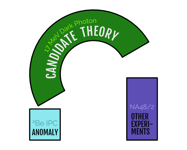
With the Atomki result was published and peer reviewed in Physics Review Letters, the game was afoot for theorists to understand how it would fit into a theoretical framework like the dark photon. A group from UC Irvine, University of Kentucky, and UC Riverside found that actually, dark photons have a hard time fitting the anomaly simultaneously with other experimental constraints. In the visual language of this recent ParticleBite, the situation was this:
It turns out that the minimal model of a dark photon cannot simultaneously explain the Atomki beryllium-8 anomaly without running afoul of other experimental constraints. Image adapted from this ParticleBite.
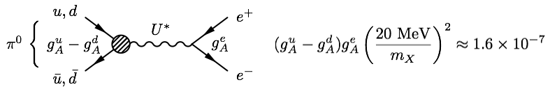
The main reason for this is that a dark photon with mass and interaction strength to fit the beryllium anomaly would necessarily have been seen by the NA48/2 experiment. This experiment looks for dark photons in the decay of neutral pions (π0). These pions typically decay into two photons, but if there’s a 17 MeV dark photon around, some fraction of those decays would go into dark-photon — ordinary-photon pairs. The non-observation of these unique decays rules out the dark photon interpretation.
The theorists then decided to “break” the dark photon theory in order to try to make it fit. They generalized the types of interactions that a new photon-like particle, X, could have, allowing protons, for example, to have completely different charges than electrons rather than having exactly opposite charges. Doing this does gross violence to the theoretical consistency of a theory—but they goal was just to see what a new particle interpretation would have to look like. They found that if a new photon-like particle talked to neutrons but not protons—that is, the new force were protophobic—then a theory might hold together.
Schematic description of how model-builders “hacked” the dark photon theory to fit both the beryllium anomaly while being consistent with other experiments. This hack isn’t pretty—and indeed, comes at the cost of potentially invalidating the mathematical consistency of the theory—but the exercise demonstrates the target for how to a complete theory might have to behave. Image adapted from this ParticleBite.
Theory appendix: pion-phobia is protophobia
Editor’s note: what follows is for readers with some physics background interested in a technical detail; others may skip this section.
How does a new particle that is allergic to protons avoid the neutral pion decay bounds from NA48/2? Pions decay into pairs of photons through the well-known triangle-diagrams of the axial anomaly. The decay into photon–dark-photon pairs proceed through similar diagrams. The goal is then to make sure that these diagrams cancel.
A cute way to look at this is to assume that at low energies, the relevant particles running in the loop aren’t quarks, but rather nucleons (protons and neutrons). In fact, since only the proton can talk to the photon, one only needs to consider proton loops. Thus if the new photon-like particle, X, doesn’t talk to protons, then there’s no diagram for the pion to decay into γX. This would be great if the story weren’t completely wrong.
Avoiding NA48/2 bounds requires that the new particle, X, is pion-phobic. It turns out that this is equivalent to X being protophobic. The correct way to see this is on the left, making sure that the contribution of up-quark loops cancels the contribution from down-quark loops. A slick (but naively completely wrong) calculation is on the right, arguing that effectively only protons run in the loop.
The correct way of seeing this is to treat the pion as a quantum superposition of an up–anti-up and down–anti-down bound state, and then make sure that the X charges are such that the contributions of the two states cancel. The resulting charges turn out to be protophobic.
The fact that the “proton-in-the-loop” picture gives the correct charges, however, is no coincidence. Indeed, this was precisely how Jack Steinberger calculated the correct pion decay rate. The key here is whether one treats the quarks/nucleons linearly or non-linearly in chiral perturbation theory. The relation to the Wess-Zumino-Witten term—which is what really encodes the low-energy interaction—is carefully explained in chapter 6a.2 of Georgi’s revised Weak Interactions.
Theory part 2: Not a spin-0 particle
The above considerations focus on a new particle with the same spin and parity as a photon (spin-1, parity odd). Another result of the UCI study was a systematic exploration of other possibilities. They found that the beryllium anomaly could not be consistent with spin-0 particles. For a parity-odd, spin-0 particle, one cannot simultaneously conserve angular momentum and parity in the decay of the excited beryllium-8 state. (Parity violating effects are negligible at these energies.)
Parity and angular momentum conservation prohibit a “dark Higgs” (parity even scalar) from mediating the anomaly.
For a parity-odd pseudoscalar, the bounds on axion-like particles at 20 MeV suffocate any reasonable coupling. Measured in terms of the pseudoscalar–photon–photon coupling (which has dimensions of inverse GeV), this interaction is ruled out down to the inverse Planck scale.
Bounds on axion-like particles exclude a 20 MeV pseudoscalar with couplings to photons stronger than the inverse Planck scale. Adapted from 1205.2671 and 1512.03069.
Additional possibilities include:
Dark Z bosons, cousins of the dark photon with spin-1 but indeterminate parity. This is very constrained by atomic parity violation.
Axial vectors, spin-1 bosons with positive parity. These remain a theoretical possibility, though their unknown nuclear matrix elements make it difficult to write a predictive model. (See section II.D of 1608.03591.)
Theory part 3: Nuclear input
The plot thickens when once also includes results from nuclear theory. Recent results from Saori Pastore, Bob Wiringa, and collaborators point out a very important fact: the 18.15 MeV beryllium-8 state that exhibits the anomaly and the 17.64 MeV state which does not are actually closely related.
Recall (e.g. from the first figure at the top) that both the 18.15 MeV and 17.64 MeV states are both spin-1 and parity-even. They differ in mass and in one other key aspect: the 17.64 MeV state carries isospin charge, while the 18.15 MeV state and ground state do not.
Isospin is the nuclear symmetry that relates protons to neutrons and is tied to electroweak symmetry in the full Standard Model. At nuclear energies, isospin charge is approximately conserved. This brings us to the following puzzle:
If the new particle has mass around 17 MeV, why do we see its effects in the 18.15 MeV state but not the 17.64 MeV state?
Naively, if the new particle emitted, X, carries no isospin charge, then isospin conservation prohibits the decay of the 17.64 MeV state through emission of an X boson. However, the Pastore et al. result tells us that actually, the isospin-neutral and isospin-charged states mix quantum mechanically so that the observed 18.15 and 17.64 MeV states are mixtures of iso-neutral and iso-charged states. In fact, this mixing is actually rather large, with mixing angle of around 10 degrees!
The result of this is that one cannot invoke isospin conservation to explain the non-observation of an anomaly in the 17.64 MeV state. In fact, the only way to avoid this is to assume that the mass of the X particle is on the heavier side of the experimentally allowed range. The rate for X emission goes like the 3-momentum cubed (see section II.E of 1608.03591), so a small increase in the mass can suppresses the rate of X emission by the lighter state by a lot.
The UCI collaboration of theorists went further and extended the Pastore et al. analysis to include a phenomenological parameterization of explicit isospin violation. Independent of the Atomki anomaly, they found that including isospin violation improved the fit for the 18.15 MeV and 17.64 MeV electromagnetic decay widths within the Pastore et al. formalism. The results of including all of the isospin effects end up changing the particle physics story of the Atomki anomaly significantly:
The rate of X emission (colored contours) as a function of the X particle’s couplings to protons (horizontal axis) versus neutrons (vertical axis). The best fit for a 16.7 MeV new particle is the dashed line in the teal region. The vertical band is the region allowed by the NA48/2 experiment. Solid lines show the dark photon and protophobic limits. Left: the case for perfect (unrealistic) isospin. Right: the case when isospin mixing and explicit violation are included. Observe that incorporating realistic isospin happens to have only a modest effect in the protophobic region. Figure from 1608.03591.
The results of the nuclear analysis are thus that:
An interpretation of the Atomki anomaly in terms of a new particle tends to push for a slightly heavier X mass than the reported best fit. (Remark: the Atomki paper does not do a combined fit for the mass and coupling nor does it report the difficult-to-quantify systematic errors associated with the fit. This information is important for understanding the extent to which the X mass can be pushed to be heavier.)
The effects of isospin mixing and violation are important to include; especially as one drifts away from the purely protophobic limit.
Theory part 4: towards a complete theory
The theoretical structure presented above gives a framework to do phenomenology: fitting the observed anomaly to a particle physics model and then comparing that model to other experiments. This, however, doesn’t guarantee that a nice—or even self-consistent—theory exists that can stretch over the scaffolding.
Indeed, a few challenges appear:
The isospin mixing discussed above means the X mass must be pushed to the heavier values allowed by the Atomki observation.
The “protophobic” limit is not obviously anomaly-free: simply asserting that known particles have arbitrary charges does not generically produce a mathematically self-consistent theory.
Atomic parity violation constraints require that the X couple in the same way to left-handed and right-handed matter. The left-handed coupling implies that X must also talk to neutrinos: these open up new experimental constraints.
The Irvine/Kentucky/Riverside collaboration first note the need for a careful experimental analysis of the actual mass ranges allowed by the Atomki observation, treating the new particle mass and coupling as simultaneously free parameters in the fit.
Next, they observe that protophobic couplings can be relatively natural. Indeed: the Standard Model Z boson is approximately protophobic at low energies—a fact well known to those hunting for dark matter with direct detection experiments. For exotic new physics, one can engineer protophobia through a phenomenon called kinetic mixing where two force particles mix into one another. A tuned admixture of electric charge and baryon number, (Q-B), is protophobic.
Baryon number, however, is an anomalous global symmetry—this means that one has to work hard to make a baryon-boson that mixes with the photon (see 1304.0576 and 1409.8165 for examples). Another alternative is if the photon kinetically mixes with not baryon number, but the anomaly-free combination of “baryon-minus-lepton number,” Q-(B-L). This then forces one to apply additional model-building modules to deal with the neutrino interactions that come along with this scenario.
In the language of the ‘model building blocks’ above, result of this process looks schematically like this:
A complete theory is completely mathematically self-consistent and satisfies existing constraints. The additional bells and whistles required for consistency make additional predictions for experimental searches. Pieces of the theory can sometimes be used to address other anomalies.
The theory collaboration presented examples of the two cases, and point out how the additional ‘bells and whistles’ required may tie to additional experimental handles to test these hypotheses. These are simple existence proofs for how complete models may be constructed.
What’s next?
We have delved rather deeply into the theoretical considerations of the Atomki anomaly. The analysis revealed some unexpected features with the types of new particles that could explain the anomaly (dark photon-like, but not exactly a dark photon), the role of nuclear effects (isospin mixing and breaking), and the kinds of features a complete theory needs to have to fit everything (be careful with anomalies and neutrinos). The single most important next step, however, is and has always been experimental verification of the result.
While the Atomki experiment continues to run with an upgraded detector, what’s really exciting is that a swath of experiments that are either ongoing or in construction will be able to probe the exact interactions required by the new particle interpretation of the anomaly. This means that the result can be independently verified or excluded within a few years. A selection of upcoming experiments is highlighted in section IX of 1608.03591:
Other experiments that can probe the new particle interpretation of the Atomki anomaly. The horizontal axis is the new particle mass, the vertical axis is its coupling to electrons (normalized to the electric charge). The dark blue band is the target region for the Atomki anomaly. Figure from 1608.03591; assuming 100% branching ratio to electrons.
We highlight one particularly interesting search: recently a joint team of theorists and experimentalists at MIT proposed a way for the LHCb experiment to search for dark photon-like particles with masses and interaction strengths that were previously unexplored. The proposal makes use of the LHCb’s ability to pinpoint the production position of charged particle pairs and the copious amounts of D mesons produced at Run 3 of the LHC. As seen in the figure above, the LHCb reach with this search thoroughly covers the Atomki anomaly region.
Implications
So where we stand is this:
There is an unexpected result in a nuclear experiment that may be interpreted as a sign for new physics.
The next steps in this story are independent experimental cross-checks; the threshold for a ‘discovery’ is if another experiment can verify these results.
Meanwhile, a theoretical framework for understanding the results in terms of a new particle has been built and is ready-and-waiting. Some of the results of this analysis are important for faithful interpretation of the experimental results.
What if it’s nothing?
This is the conservative take—and indeed, we may well find that in a few years, the possibility that Atomki was observing a new particle will be completely dead. Or perhaps a source of systematic error will be identified and the bump will go away. That’s part of doing science.
Meanwhile, there are some important take-aways in this scenario. First is the reminder that the search for light, weakly coupled particles is an important frontier in particle physics. Second, for this particular anomaly, there are some neat take aways such as a demonstration of how effective field theory can be applied to nuclear physics (see e.g. chapter 3.1.2 of the new book by Petrov and Blechman) and how tweaking our models of new particles can avoid troublesome experimental bounds. Finally, it’s a nice example of how particle physics and nuclear physics are not-too-distant cousins and how progress can be made in particle–nuclear collaborations—one of the Irvine group authors (Susan Gardner) is a bona fide nuclear theorist who was on sabbatical from the University of Kentucky.
What if it’s real?
This is a big “what if.” On the other hand, a 6.8σ effect is not a statistical fluctuation and there is no known nuclear physics to produce a new-particle-like bump given the analysis presented by the Atomki experimentalists.
The threshold for “real” is independent verification. If other experiments can confirm the anomaly, then this could be a huge step in our quest to go beyond the Standard Model. While this type of particle is unlikely to help with the Hierarchy problem of the Higgs mass, it could be a sign for other kinds of new physics. One example is the grand unification of the electroweak and strong forces; some of the ways in which these forces unify imply the existence of an additional force particle that may be light and may even have the types of couplings suggested by the anomaly.
Could it be related to other anomalies?
The Atomki anomaly isn’t the first particle physics curiosity to show up at the MeV scale. While none of these other anomalies are necessarily related to the type of particle required for the Atomki result (they may not even be compatible!), it is helpful to remember that the MeV scale may still have surprises in store for us.
The KTeV anomaly: The rate at which neutral pions decay into electron–positron pairs appears to be off from the expectations based on chiral perturbation theory. In 0712.0007, a group of theorists found that this discrepancy could be fit to a new particle with axial couplings. If one fixes the mass of the proposed particle to be 20 MeV, the resulting couplings happen to be in the same ballpark as those required for the Atomki anomaly. The important caveat here is that parameters for an axial vector to fit the Atomki anomaly are unknown, and mixed vector–axial states are severely constrained by atomic parity violation.
The KTeV anomaly interpreted as a new particle, U. From 0712.0007.
The anomalous magnetic moment of the muon and the cosmic lithium problem: much of the progress in the field of light, weakly coupled forces comes from Maxim Pospelov. The anomalous magnetic moment of the muon, (g-2)μ, has a long-standing discrepancy from the Standard Model (see e.g. this blog post). While this may come from an error in the very, very intricate calculation and the subtle ways in which experimental data feed into it, Pospelov (and also Fayet) noted that the shift may come from a light (in the 10s of MeV range!), weakly coupled new particle like a dark photon. Similarly, Pospelov and collaborators showed that a new light particle in the 1-20 MeV range may help explain another longstanding mystery: the surprising lack of lithium in the universe (APS Physics synopsis).
The Proton Radius Problem: the charge radius of the proton appears to be smaller than expected when measured using the Lamb shift of muonic hydrogen versus electron scattering experiments. See this ParticleBite summary, and this recent review. Some attempts to explain this discrepancy have involved MeV-scale new particles, though the endeavor is difficult. There’s been some renewed popular interest after a new result using deuterium confirmed the discrepancy. However, there was a report that a result at the proton radius problem conference in Trento suggests that the 2S-4P determination of the Rydberg constant may solve the puzzle (though discrepant with other Rydberg measurements). [Those slides do not appear to be public.]
Could it be related to dark matter?
A lot of recent progress in dark matter has revolved around the possibility that in addition to dark matter, there may be additional light particles that mediate interactions between dark matter and the Standard Model. If these particles are light enough, they can change the way that we expect to find dark matter in sometimes surprising ways. One interesting avenue is called self-interacting dark matter and is based on the observation that these light force carriers can deform the dark matter distribution in galaxies in ways that seem to fit astronomical observations. A 20 MeV dark photon-like particle even fits the profile of what’s required by the self-interacting dark matter paradigm, though it is very difficult to make such a particle consistent with both the Atomki anomaly and the constraints from direct detection.
Should I be excited?
Given all of the caveats listed above, some feel that it is too early to be in “drop everything, this is new physics” mode. Others may take this as a hint that’s worth exploring further—as has been done for many anomalies in the recent past. For researchers, it is prudent to be cautious, and it is paramount to be careful; but so long as one does both, then being excited about a new possibility is part what makes our job fun.
For the general public, the tentative hopes of new physics that pop up—whether it’s the Atomki anomaly, or the 750 GeV diphoton bump, a GeV bump from the galactic center, γ-ray lines at 3.5 keV and 130 GeV, or penguins at LHCb—these are the signs that we’re making use of all of the data available to search for new physics. Sometimes these hopes fizzle away, often they leave behind useful lessons about physics and directions forward. Maybe one of these days an anomaly will stick and show us the way forward.
Further Reading
Here are some of the popular-level press on the Atomki result. See the references at the top of this ParticleBite for references to the primary literature.


 to prove the result:


