Daya Bay and the search for sterile neutrinos

Article: Improved search for a light sterile neutrino with the full configuration of the Daya Bay Experiment
Authors: Daya Bay Collaboration
Reference: arXiv:1607.01174

Today I bring you news from the Daya Bay reactor neutrino experiment, which detects neutrinos emitted by three nuclear power plants on the southern coast of China. The results in this paper are based on the first 621 days of data, through November 2013; more data remain to be analyzed, and we can expect a final result after the experiment ends in 2017.

Figure 1: Antineutrino detectors installed in the far hall of the Daya Bay experiment. Source: LBL news release.

For more on sterile neutrinos, see also this recent post by Eve.

Neutrino oscillations

Neutrinos exist in three flavors, each corresponding to one of the charged leptons: electron neutrinos (\nu_e), muon neutrinos (\nu_\mu) and tau neutrinos (\nu_\tau). When a neutrino is born via the weak interaction, it is created in a particular flavor eigenstate. So, for example, a neutrino born in the sun is always an electron neutrino. However, the electron neutrino does not have a definite mass. Instead, each flavor eigenstate is a linear combination of the three mass eigenstates. This “mixing” of the flavor and mass eigenstates is described by the PMNS matrix, as shown in Figure 2.

Figure 2: Each neutrino flavor eigenstate is a linear combination of the three mass eigenstates.

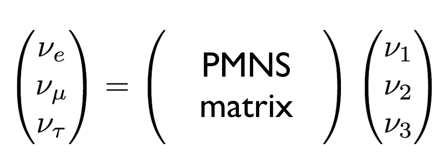
The PMNS matrix can be parameterized by 4 numbers: three mixing angles (θ12, θ23 and θ13) and a phase (δ).1  These parameters aren’t known a priori — they must be measured by experiments.

Solar neutrinos stream outward in all directions from their birthplace in the sun. Some intercept Earth, where human-built neutrino observatories can inventory their flavors. After traveling 150 million kilometers, only ⅓ of them register as electron neutrinos — the other ⅔ have transformed along the way into muon or tau neutrinos. These neutrino flavor oscillations are the experimental signature of neutrino mixing, and the means by which we can tease out the values of the PMNS parameters. In any specific situation, the probability of measuring each type of neutrino  is described by some experiment-specific parameters (the neutrino energy, distance from the source, and initial neutrino flavor) and some fundamental parameters of the theory (the PMNS mixing parameters and the neutrino mass-squared differences). By doing a variety of measurements with different neutrino sources and different source-to-detector (“baseline”) distances, we can attempt to constrain or measure the individual theory parameters. This has been a major focus of the worldwide experimental neutrino program for the past 15 years.

1 This assumes the neutrino is a Dirac particle. If the neutrino is a Majorana particle, there are two more phases, for a total of 6 parameters in the PMNS matrix.

Sterile neutrinos

Many neutrino experiments have confirmed our model of neutrino oscillations and the existence of three neutrino flavors. However, some experiments have observed anomalous signals which could be explained by the presence of a fourth neutrino. This proposed “sterile” neutrino doesn’t have a charged lepton partner (and therefore doesn’t participate in weak interactions) but does mix with the other neutrino flavors.

The discovery of a new type of particle would be tremendously exciting, and neutrino experiments all over the world (including Daya Bay) have been checking their data for any sign of sterile neutrinos.

Neutrinos from reactors

Figure 3: Chart of the nuclides, color-coded by decay mode. Source: modified from Wikimedia Commons.

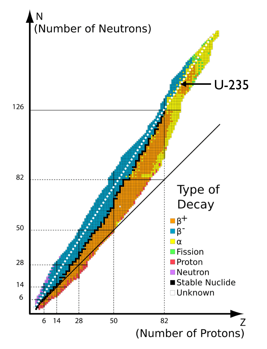
Nuclear reactors are a powerful source of electron antineutrinos. To see why, take a look at this zoomed out version of the chart of the nuclides. The chart of the nuclides is a nuclear physicist’s version of the periodic table. For a chemist, Hydrogen-1 (a single proton), Hydrogen-2 (one proton and one neutron) and Hydrogen-3 (one proton and two neutrons) are essentially the same thing, because chemical bonds are electromagnetic and every hydrogen nucleus has the same electric charge. In the realm of nuclear physics, however, the number of neutrons is just as important as the number of protons. Thus, while the periodic table has a single box for each chemical element, the chart of the nuclides has a separate entry for every combination of protons and neutrons (“nuclide”) that has ever been observed in nature or created in a laboratory.

The black squares are stable nuclei. You can see that stability only occurs when the ratio of neutrons to protons is just right. Furthermore, unstable nuclides tend to decay in such a way that the daughter nuclide is closer to the line of stability than the parent.

Nuclear power plants generate electricity by harnessing the energy released by the fission of Uranium-235. Each U-235 nucleus contains 143 neutrons and 92 protons (n/p = 1.6). When U-235 undergoes fission, the resulting fragments also have n/p ~ 1.6, because the overall number of neutrons and protons is still the same. Thus, fission products tend to lie along the white dashed line in Figure 3, which falls above the line of stability. These nuclides have too many neutrons to be stable, and therefore undergo beta decay: n \to p + e + \bar{\nu}_e. A typical power reactor emits 6 × 10^20 \bar{\nu}_e per second.

Figure 4: Layout of the Daya Bay experiment. Source: arXiv:1508.03943.

The Daya Bay experiment

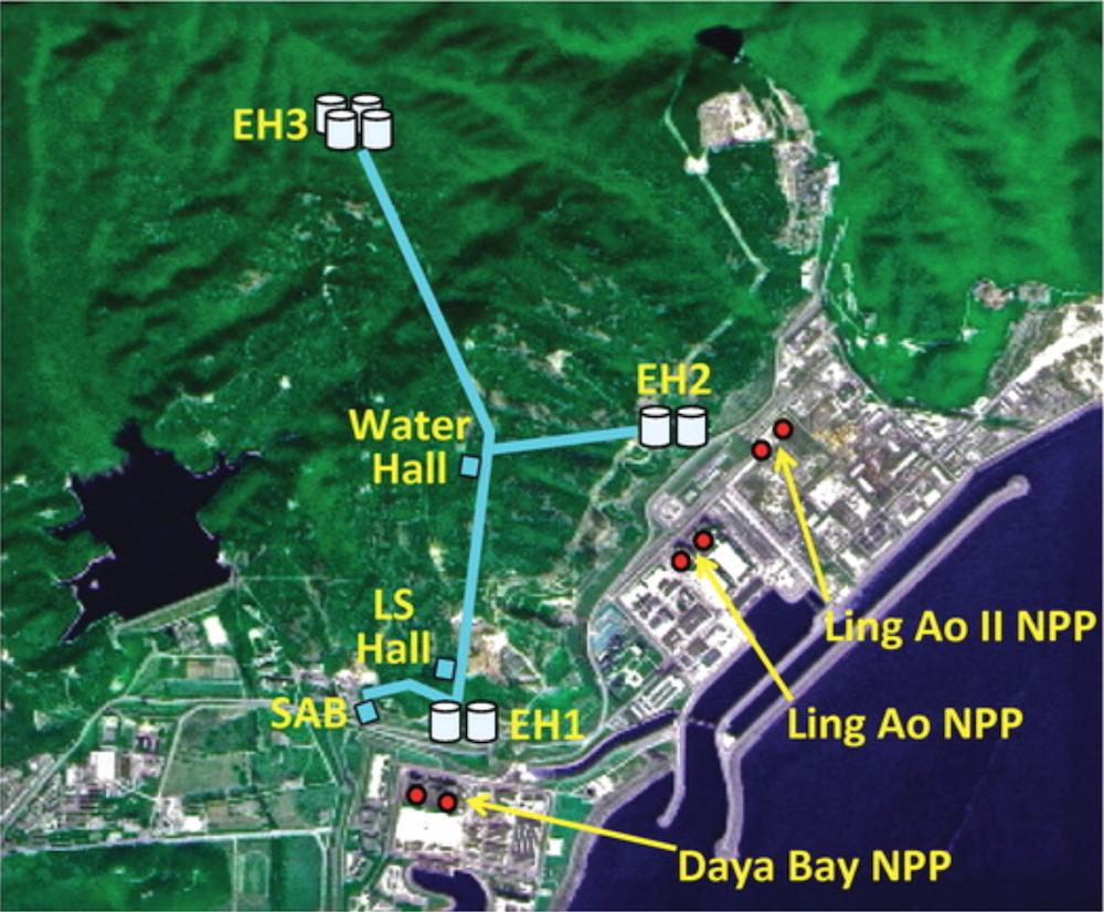
The Daya Bay nuclear power complex is located on the southern coast of China, 55 km northeast of Hong Kong. With six reactor cores, it is one of the most powerful reactor complexes in the world — and therefore an excellent source of electron antineutrinos. The Daya Bay experiment consists of 8 identical antineutrino detectors in 3 underground halls. One experimental hall is located as close as possible to the Daya Bay nuclear power plant; the second is near the two Ling Ao power plants; the third is located 1.5 – 1.9 km away from all three pairs of reactors, a distance chosen to optimize Daya Bay’s sensitivity to the mixing angle \theta_{13}.

The neutrino target at the heart of each detector is a cylindrical vessel filled with 20 tons of Gadolinium-doped liquid scintillator. The vast majority of \bar{\nu}_e pass through undetected, but occasionally one will undergo inverse beta decay in the target volume, interacting with a proton to produce a positron and a neutron: \bar{\nu}_e + p \to e^+ + n.

Figure 5: Design of the Daya Bay \bar{\nu}_e 
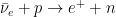
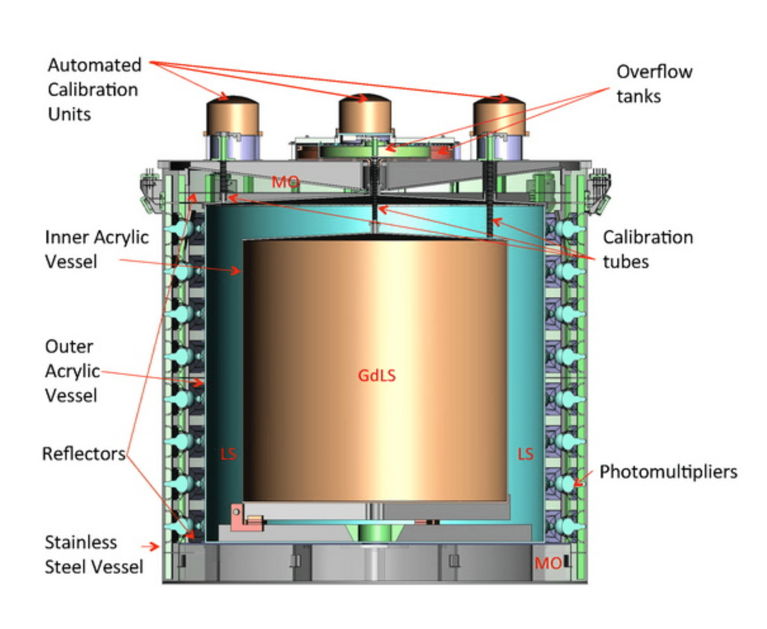
detectors. Each detector consists of three nested cylindrical vessels. The inner acrylic vessel is about 3 meters tall and 3 meters in diameter. It contains 20 tons of Gadolinium-doped liquid scintillator; when a \bar{\nu}_e interacts in this volume, the resulting signal can be picked up by the detector. The outer acrylic vessel holds an additional 22 tons of liquid scintillator; this layer exists so that \bar{\nu}_e interactions near the edge of the inner volume are still surrounded by scintillator on all sides — otherwise, some of the gamma rays produced in the event might escape undetected. The stainless steel outer vessel is filled with 40 tons of mineral oil; its purpose to prevent outside radiation from reaching the scintillator. Finally, the outer vessel is lined with 192 photomultiplier tubes, which collect the scintillation light produced by particle interactions in the active scintillation volumes. The whole device is underwater for additional shielding. Source: arXiv:1508.03943.
Figure 6: Cartoon version of the signal produced in the Daya Bay detectors by inverse beta decay. The size of the prompt pulse is related to the antineutrino energy; the delayed pulse has a characteristic energy of 8 MeV.

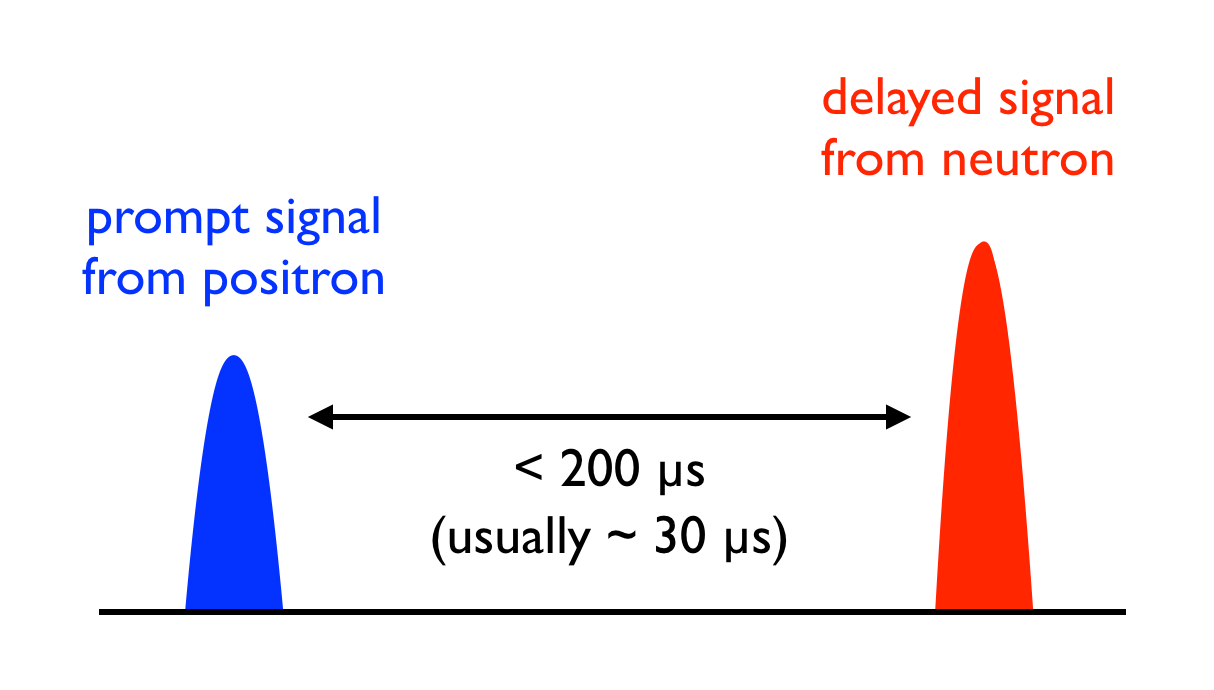
The positron and neutron create signals in the detector with a characteristic time relationship, as shown in Figure 6. The positron immediately deposits its energy in the scintillator and then annihilates with an electron. This all happens within a few nanoseconds and causes a prompt flash of scintillation light. The neutron, meanwhile, spends some tens of microseconds bouncing around (“thermalizing”) until it is slow enough to be captured by a Gadolinium nucleus. When this happens, the nucleus emits a cascade of gamma rays, which in turn interact with the scintillator and produce a second flash of light. This combination of prompt and delayed signals is used to identify \bar{\nu}_e interaction events.

Daya Bay’s search for sterile neutrinos

Daya Bay is a neutrino disappearance experiment. The electron antineutrinos emitted by the reactors can oscillate into muon or tau antineutrinos as they travel, but the detectors are only sensitive to \bar{\nu}_e, because the antineutrinos have enough energy to produce a positron but not the more massive \mu^+ or \tau^+. Thus, Daya Bay observes neutrino oscillations by measuring fewer \bar{\nu}_e than would be expected otherwise.

Based on the number of \bar{\nu}_e detected at one of the Daya Bay experimental halls, the usual three-neutrino oscillation theory can predict the number that will be seen at the other two experimental halls (EH). You can see how this plays out in Figure 7. We are looking at the neutrino energy spectrum measured at EH2 and EH3, divided by the prediction computed from the EH1 data. The gray shaded regions mark the one-standard-deviation uncertainty bounds of the predictions. If the black data points deviated significantly from the shaded region, that would be a sign that the three-neutrino oscillation model is not complete, possibly due to the presence of sterile neutrinos. However, in this case, the black data points are statistically consistent with the prediction. In other words, Daya Bay sees no evidence for sterile neutrinos.

Figure 7: Some results of the Daya Bay sterile neutrino search. Source: arxiv:1607.01174.

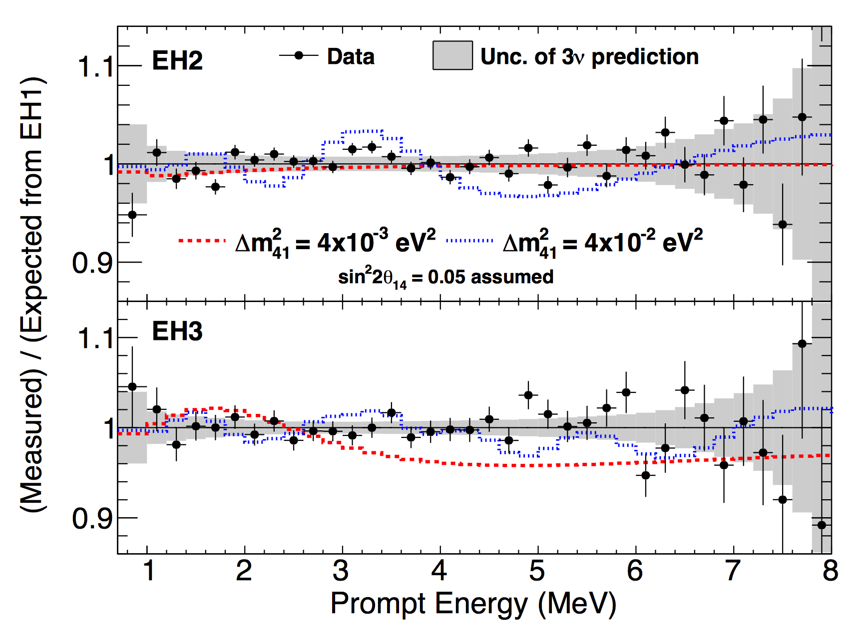
Does that mean sterile neutrinos don’t exist? Not necessarily. For one thing, the effect of a sterile neutrino on the Daya Bay results would depend on the sterile neutrino mass and mixing parameters. The blue and red dashed lines in Figure 7 show the sterile neutrino prediction for two specific choices of \theta_{14} and \Delta m_{41}^2; these two examples look quite different from the three-neutrino prediction and can be ruled out because they don’t match the data. However, there are other parameter choices for which the presence of a sterile neutrino wouldn’t have a discernable effect on the Daya Bay measurements. Thus, Daya Bay can constrain the parameter space, but can’t rule out sterile neutrinos completely. However, as more and more experiments report “no sign of sterile neutrinos here,” it appears less and less likely that they exist.

Further Reading

A new anomaly: the electromagnetic duality anomaly

Article: Electromagnetic duality anomaly in curved spacetimes
Authors: I. Agullo, A. del Rio and J. Navarro-Salas
Reference: arXiv:1607.08879

Disclaimer: this blogpost requires some basic knowledge of QFT (or being comfortable with taking my word at face value for some of the claims made :))

Anomalies exists everywhere. Probably the most intriguing ones are medical, but in particle physics they can be pretty fascinating too. In physics, anomalies refer to the breaking of a symmetry. There are basically two types of anomalies:

  • The first type, gauge anomalies, are red-flags: if they show up in your theory, they indicate that the theory is mathematically inconsistent.
  • The second type of anomaly does not signal any problems with the theory and in fact can have experimentally observable consequences. A prime example is the chiral anomaly. This anomaly nicely explains the decay rate of the neutral pion into two photons.
    Fig. 1: Illustration of pion decay into two photons. [Credit: Wikimedia Commons]

In this paper, a new anomaly is discussed. This anomaly is related to the polarization of light and is called the electromagnetic duality anomaly.

Chiral anomaly 101
So let’s first brush up on the basics of the chiral anomaly. How does this anomaly explain the decay rate of the neutral pion into two photons? For that we need to start with the Lagrangian for QED that describes the interactions between the electromagnetic field (that is, the photons) and spin-½ fermions (which pions are build from):

\displaystyle \mathcal L = \bar\psi \left( i \gamma^\mu \partial_\mu - i e \gamma^\mu A_\mu \right) \psi + m \bar\psi \psi

where the important players in the above equation are the \psis that describe the spin-½ particles and the vector potential A_\mu that describes the electromagnetic field. This Lagrangian is invariant under the chiral symmetry:

\displaystyle \psi \to e^{i \gamma_5} \psi .

Due to this symmetry the current density j^\mu = \bar{\psi} \gamma_5 \gamma^\mu \psi is conserved: \nabla_\mu j^\mu = 0. This then immediately tells us that the charge associated with this current density is time-independent. Since the chiral charge is time-independent, it prevents the \psi fields to decay into the electromagnetic fields, because the \psi field has a non-zero chiral charge and the photons have no chiral charge. Hence, if this was the end of the story, a pion would never be able to decay into two photons.

However, the conservation of the charge is only valid classically! As soon as you go from classical field theory to quantum field theory this is no longer true; hence, the name (quantum) anomaly.  This can be seen most succinctly using Fujikawa’s observation that even though the field \psi and Lagrangian are invariant under the chiral symmetry, this is not enough for the quantum theory to also be invariant. If we take the path integral approach to quantum field theory, it is not just the Lagrangian that needs to be invariant but the entire path integral needs to be:

\displaystyle \int D[A] \, D[\bar\psi]\, \int D[\psi] \, e^{i\int d^4x \mathcal L} .

From calculating how the chiral symmetry acts on the measure D \left[\psi \right]  \, D \left[\bar \psi \right], one can extract all the relevant physics such as the decay rate.

The electromagnetic duality anomaly
Just like the chiral anomaly, the electromagnetic duality anomaly also breaks a symmetry at the quantum level that exists classically. The symmetry that is broken in this case is – as you might have guessed from its name – the electromagnetic duality. This symmetry is a generalization of a symmetry you are already familiar with from source-free electromagnetism. If you write down source-free Maxwell equations, you can just swap the electric and magnetic field and the equations look the same (you just have to send  \displaystyle \vec{E} \to \vec{B} and \vec{B} \to - \vec{E}). Now the more general electromagnetic duality referred to here is slightly more difficult to visualize: it is a rotation in the space of the electromagnetic field tensor and its dual. However, its transformation is easy to write down mathematically:

\displaystyle F_{\mu \nu} \to \cos \theta \, F_{\mu \nu} + \sin \theta \, \, ^\ast F_{\mu \nu} .

In other words, since this is a symmetry, if you plug this transformation into the Lagrangian of electromagnetism, the Lagrangian will not change: it is invariant. Now following the same steps as for the chiral anomaly, we find that the associated current is conserved and its charge is time-independent due to the symmetry. Here, the charge is simply the difference between the number of photons with left helicity and those with right helicity.

Let us continue following the exact same steps as those for the chiral anomaly. The key is to first write electromagnetism in variables analogous to those of the chiral theory. Then you apply Fujikawa’s method and… *drum roll for the anomaly that is approaching*…. Anti-climax: nothing happens, everything seems to be fine. There are no anomalies, nothing!

So why the title of this blog? Well, as soon as you couple the electromagnetic field with a gravitational field, the electromagnetic duality is broken in a deeply quantum way. The number of photon with left helicity and right helicity is no longer conserved when your spacetime is curved.

Physical consequences
Some potentially really cool consequences have to do with the study of light passing by rotating stars, black holes or even rotating clusters. These astrophysical objects do not only gravitationally bend the light, but the optical helicity anomaly tells us that there might be a difference in polarization between lights rays coming from different sides of these objects. This may also have some consequences for the cosmic microwave background radiation, which is ‘picture’ of our universe when it was only 380,000 years old (as compared to the 13.8 billion years it is today!). How big this effect is and whether we will be able to see it in the near future is still an open question.


Further reading 

  • An introduction to anamolies using only quantum mechanics instead of quantum field theory is “Anomalies for pedestrians” by Barry Holstein 
  • The beautiful book “Quantum field theory and the Standard Model” by Michael Schwartz has a nice discussion in the later chapters on the chiral anomaly.
  • Lecture notes by Adal Bilal for graduate students on anomalies in general  can be found here

Horton Hears a Sterile Neutrino?

Article: Limits on Active to Sterile Neutrino Oscillations from Disappearance Searches in the MINOS, Daya Bay, and Bugey-3 Experiments
Authors:  Daya Bay and MINOS collaborations
Reference: arXiv:1607.01177v4

So far, the hunt for sterile neutrinos has come up empty. Could a joint analysis between MINOS, Daya Bay and Bugey-3 data hint at their existence?

Neutrinos, like the beloved Whos in Dr. Seuss’ “Horton Hears a Who!,” are light and elusive, yet have a large impact on the universe we live in. While neutrinos only interact with matter through the weak nuclear force and gravity, they played a critical role in the formation of the early universe. Neutrino physics is now an exciting line of research pursued by the Hortons of particle physics, cosmology, and astrophysics alike. While most of what we currently know about neutrinos is well described by a three-flavor neutrino model, a few inconsistent experimental results such as those from the Liquid Scintillator Neutrino Detector (LSND) and the Mini Booster Neutrino Experiment (MiniBooNE) hint at the presence of a new kind of neutrino that only interacts with matter through gravity. If this “sterile” kind of neutrino does in fact exist, it might also have played an important role in the evolution of our universe.

Horton hears a sterile neutrino? Source: imdb.com

The three known neutrinos come in three flavors: electron, muon, or tau. The discovery of neutrino oscillation by the Sudbury Neutrino Observatory and the Super-Kamiokande Observatory, which won the 2015 Nobel Prize, proved that one flavor of neutrino can transform into another. This led to the realization that each neutrino mass state is a superposition of the three different neutrino flavor states. From neutrino oscillation measurements, most of the parameters that define the mixing between neutrino states are well known for the three standard neutrinos.

The relationship between the three known neutrino flavor states and mass states is usually expressed as a 3×3 matrix known as the PMNS matrix, for Bruno Pontecorvo, Ziro Maki, Masami Nakagawa and Shoichi Sakata. The PMNS matrix includes three mixing angles, the values of which determine “how much” of each neutrino flavor state is in each mass state. The distance required for one neutrino flavor to become another, the neutrino oscillation wavelength, is determined by the difference between the squared masses of the two mass states. The values of mass splittings m_2^2-m_1^2 and m_3^2-m_2^2 are known to good precision.

A fourth flavor? Adding a sterile neutrino to the mix

A “sterile” neutrino is referred to as such because it would not interact weakly: it would only interact through the gravitational force. Neutrino oscillations involving the hypothetical sterile neutrino can be understood using a “four-flavor model,” which introduces a fourth neutrino mass state, m_4, heavier than the three known “active” mass states. This fourth neutrino state would be mostly sterile, with only a small contribution from a mixture of the three known neutrino flavors. If the sterile neutrino exists, it should be possible to experimentally observe neutrino oscillations with a wavelength set by the difference between m_4^2 and the square of the mass of another known neutrino mass state. Current observations suggest a squared mass difference in the range of 0.1-10 eV^2.

Oscillations between active and sterile states would result in the disappearance of muon (anti)neutrinos and electron (anti)neutrinos. In a disappearance experiment, you know how many neutrinos of a specific type you produce, and you count the number of that type of neutrino a distance away, and find that some of the neutrinos have “disappeared,” or in other words, oscillated into a different type of neutrino that you are not detecting.

A joint analysis by the MINOS and Daya Bay collaborations

The MINOS and Daya Bay collaborations have conducted a joint analysis to combine independent measurements of muon (anti)neutrino disappearance by MINOS and electron antineutrino disappearance by Daya Bay and Bugey-3. Here’s a breakdown of the involved experiments:

  • MINOS, the Main Injector Neutrino Oscillation Search: A long-baseline neutrino experiment with detectors at Fermilab and northern Minnesota that use an accelerator at Fermilab as the neutrino source
  • The Daya Bay Reactor Neutrino Experiment: Uses antineutrinos produced by the reactors of China’s Daya Bay Nuclear Power Plant and the Ling Ao Nuclear Power Plant
  • The Bugey-3 experiment: Performed in the early 1990s, used antineutrinos from the Bugey Nuclear Power Plant in France for its neutrino oscillation observations
Screen Shot 2016-09-12 at 10.22.49 AM
MINOS and Daya Bay/Bugey-3 combined 90% confidence level limits (in red) compared to the LSND and MiniBooNE 90% confidence level allowed regions (in green/purple). Plots the mass splitting between mass states 1 and 4 (corresponding to the sterile neutrino) against a function of the \mu-e mixing angle, which is equivalent to a function involving the 1-4 and 2-4 mixing angles. Regions of parameter space to the right of the red contour are excluded, counting out the majority of the LSND/MiniBooNE allowed regions. Source: arXiv:1607.01177v4.

Assuming a four-flavor model, the MINOS and Daya Bay collaborations put new constraints on the value of the mixing angle \theta_{\mu e}, the parameter controlling electron (anti)neutrino appearance in experiments with short neutrino travel distances. As for the hypothetical sterile neutrino? The analysis excluded the parameter space allowed by the LSND and MiniBooNE appearance-based indications for the existence of light sterile neutrinos for \Delta m_{41}^2 < 0.8 eV^2 at a 95% confidence level. In other words, the MINOS and Daya Bay analysis essentially rules out the LSND and MiniBooNE inconsistencies that allowed for the presence of a sterile neutrino in the first place. These results illustrate just how at odds disappearance searches and appearance searches are when it comes to providing insight into the existence of light sterile neutrinos. If the Whos exist, they will need to be a little louder in order for the world to hear them.


Background reading:

Inspecting the Higgs with a golden probe

Hello particle nibblers,

After recovering from a dead-diphoton-excess induced depression (see here, here, and here for summaries) I am back to tell you a little more about something that actually does exist, our old friend Monsieur Higgs boson. All of the fuss over the past few months over a potential new particle at 750 GeV has perhaps made us forget just how special and interesting the Higgs boson really is, but as more data is collected at the LHC, we will surely be reminded of this fact once again (see Fig.1).

Figure 1: Monsieur Higgs boson struggles to understand the Higgs mechanism.

Previously I discussed how one of the best and most precise ways to study the Higgs boson is just by `shining light on it’, or more specifically via its decays to pairs of photons. Today I want to expand on another fantastic and precise way to study the Higgs which I briefly mentioned previously; Higgs decays to four charged leptons (specifically electrons and muons) shown in Fig.2. This is a channel near and dear to my heart and has a long history because it was realized, way before the Higgs was actually discovered at 125 GeV, to be among the best ways to find a Higgs boson over a large range of potential masses above around 100 GeV. This led to it being dubbed the “gold plated” Higgs discovery mode, or “golden channel”, and in fact was one of the first channels (along with the diphoton channel) in which the 125 GeV Higgs boson was discovered at the LHC.

Figure 2: Higgs decays to four leptons are mediated by the various physics effects which can enter in the grey blob. Could new physics be hiding in there?

One of the characteristics that makes the golden channel so valuable as a probe of the Higgs is that it is very precisely measured by the ATLAS and CMS experiments and has a very good signal to background ratio. Furthermore, it is very well understood theoretically since most of the dominant contributions can be calculated explicitly for both the signal and background. The final feature of the golden channel that makes it valuable, and the one that I will focus on today, is that it contains a wealth of information in each event due to the large number of observables associated with the four final state leptons.

Since there are four charged leptons which are measured and each has an associated four momentum, there are in principle 16 separate numbers which can be measured in each event. However, the masses of the charged leptons are tiny in comparison to the Higgs mass so we can consider them as massless (see Footnote 1) to a very good approximation. This then reduces (using energy-momentum conservation) the number of observables to 12 which, in the lab frame, are given by the transverse momentum, rapidity, and azimuthal angle of each lepton. Now, Lorentz invariance tells us that physics doesnt care which frame of reference we pick to analyze the four lepton system. This allows us to perform a Lorentz transformation from the lab frame where the leptons are measured, but where the underlying physics can be obscured, to the much more convenient and intuitive center of mass frame of the four lepton system. Due to energy-momentum conservation, this is also the center of mass frame of the Higgs boson. In this frame the Higgs boson is at rest and the \emph{pairs} of leptons come out back to back (see Footnote 2) .

In this frame the 12 observables can be divided into 4 production and 8 decay (see Footnote 3). The 4 production variables are characterized by the transverse momentum (which has two components), the rapidity, and the azimuthal angle of the four lepton system. The differential spectra for these four variables (especially the transverse momentum and rapidity) depend very much on how the Higgs is produced and are also affected by parton distribution functions at hadron colliders like the LHC. Thus the differential spectra for these variables can not in general be computed explicitly for Higgs production at the LHC.

The 8 decay observables are characterized by the center of mass energy of the four lepton system, which in this case is equal to the Higgs mass, as well as two invariant masses associated with each pair of leptons (how one picks the pairs is arbitrary). There are also five angles (\Theta, \theta_1, \theta_2, Φ, Φ1) shown in Fig. 3 for a particular choice of lepton pairings. The angle \Theta is defined as the angle between the beam axis (labeled by p or z) and the axis defined to be in the direction of the momentum of one of the lepton pair systems (labeled by Z1 or z’). This angle also defines the ‘production plane’. The angles \theta_1, \theta_2 are the polar angles defined in the lepton pair rest frames. The angle Φ1 is the azimuthal angle between the production plane and the plane formed from the four vectors of one of the lepton pairs (in this case the muon pair). Finally Φ is defined as the azimuthal angle between the decay planes formed out of the two lepton pairs.

Figure 3: Angular center of mass observables ($latex \Theta, \theta_1, \theta_2, Φ, Φ_1$) in Higgs to four lepton decays.
Figure 3: Angular center of mass observables in Higgs to four lepton decays.

To a good approximation these decay observables are independent of how the Higgs boson is produced. Furthermore, unlike the production variables, the fully differential spectra for the decay observables can be computed explicitly and even analytically. Each of them contains information about the properties of the Higgs boson as do the correlations between them. We see an example of this in Fig. 4 where we show the one dimensional (1D) spectrum for the Φ variable under various assumptions about the CP properties of the Higgs boson.

Figure 4: Here I show various examples for the Φ differential spectrum assuming different possibilities for the CP properties of the Higgs boson.

This variable has long been known to be sensitive to the CP properties of the Higgs boson. An effect like CP violation would show up as an asymmetry in this Φ distribution which we can see in curve number 5 shown in orange. Keep in mind though that although I show a 1D spectrum for Φ, the Higgs to four lepton decay is a multidimensional differential spectrum of the 8 decay observables and all of their correlations. Thus though we can already see from a 1D projection for Φ how information about the Higgs is contained in these distributions, MUCH more information is contained in the fully differential decay width of Higgs to four lepton decays. This makes the golden channel a powerful probe of the detailed properties of the Higgs boson.

OK nibblers, hopefully I have given you a flavor of the golden channel and why it is valuable as a probe of the Higgs boson. In a future post I will discuss in more detail the various types of physics effects which can enter in the grey blob in Fig. 2. Until then, keep nibbling and don’t let dead diphotons get you down!

Footnote 1: If you are feeling uneasy about the fact that the Higgs can only “talk to” particles with mass and yet can decay to four massless (atleast approximately) leptons, keep in mind they do not interact directly. The Higgs decay to four charged leptons is mediated by intermediate particles which DO talk to the Higgs and charged leptons.

Footnote 2: More precisely, in the Higgs rest frame, the four vector formed out of the sum of the two four vectors of any pair of leptons which are chosen will be back to back with the four vector formed out of the sum of the second pair of leptons.

Footnote 3: This dividing into production and decay variables after transforming to the four lepton system center of mass frame (i.e. Higgs rest frame) is only possible in practice because all four leptons are visible and their four momentum can be reconstructed with very good precision at the LHC. This then allows for the rest frame of the Higgs boson to be reconstructed on an event by event basis. For final states with missing energy or jets which can not be reconstructed with high precision, transforming to the Higgs rest frame is in general not possible.

Dragonfly 44: A potential Dark Matter Galaxy

Title: A High Stellar Velocity Dispersion and ~100 Globular Clusters for the Ultra Diffuse Galaxy Dragonfly 44

PublicationApJ, v828, Number 1, arXiv: 1606.06291

The title of this paper sounds like some standard astrophysics analyses; but, dig a little deeper and you’ll find – what I think – is an incredibly interesting, surprising and unexpected observation.

The Coma Cluster: NASA, ESA, and the Hubble Heritage Team (STScI/AURA)

Last year, using the WM Keck Observatory and the Gemini North Telescope in Manuakea, Hawaii, the Dragonfly Telephoto Array observed the Coma cluster (a large cluster of galaxies in the constellation Coma – I’ve included a Hubble Image to the left). The team identified a population of large, very low surface brightness (ie: not a lot of stars), spheroidal galaxies around an Ultra Diffuse Galaxy (UDG) called Dragonfly 44 (shown below). They determined that Dragonfly 44 has so few stars that gravity could not hold it together – so some other matter had to be involved – namely DARK MATTER (my favorite kind of unknown matter).


The ultra-diffuse galaxy Dragonfly 44. The galaxy consists almost entirely of dark matter. It is surrounded by faint, compact sources. Image credit: Pieter van Dokkum / Roberto Abraham / Gemini Observatory / SDSS / AURA.
The ultra-diffuse galaxy Dragonfly 44. The galaxy consists almost entirely of dark matter. It is surrounded by faint, compact sources. Image credit: Pieter van Dokkum / Roberto Abraham / Gemini Observatory / SDSS / AURA

The team used the DEIMOS instrument installed on Keck II to measure the velocities of stars for 33.5 hours over a period of six nights so they could determine the galaxy’s mass. Observations of Dragonfly 44’s rotational speed suggest that it has a mass of about one trillion solar masses, about the same as the Milky Way. However, the galaxy emits only 1% of the light emitted by the Milky Way. In other words, the Milky Way has more than a hundred times more stars than Dragonfly 44. I’ve also included the Mass-to-Light ratio plot vs. the dynamical mass. This illustrates how unique Dragonfly 44 is compared to other dark matter dominated galaxies like dwarf spheroidal galaxies.


MLratio
Relation between dynamical mass-to-light ratio and dynamical mass. Open symbols are dispersion-dominated objects from Zaritsky, Gonzalez, & Zabludoff (2006) and Wolf et al. (2010). The UDGs VCC 1287 (Beasley et al. 2016) and Dragonfly 44 fall outside of the band defined by the other galaxies, having a very high M/L ratio for their mass.

What is particularly exciting is that we don’t understand how galaxies like this form.

Their research indicates that these UDGs could be failed galaxies, with the sizes, dark matter content, and globular cluster systems of much more luminous objects. But we’ll need to discover more to fully understand them.


Further reading (works by the same authors)
Forty-Seven Milky Way-Sized, Extremely Diffuse Galaxies in the Coma Cluster,arXiv: 1410.8141
Spectroscopic Confirmation of the Existence of Large, Diffuse Galaxies in the Coma Cluster: arXiv: 1504.03320

Searching for Magnetic Monopoles with MoEDAL

Article: Search for magnetic monopoles with the MoEDAL prototype trapping detector in 8 TeV proton-proton collisions at the LHC
Authors: The ATLAS Collaboration
Reference:  arXiv:1604.06645v4 [hep-ex]

Somewhere in a tiny corner of the massive LHC cavern, nestled next to the veteran LHCb detector, a new experiment is coming to life.

The Monopole & Exotics Detector at the LHC, nicknamed the MoEDAL experiment, recently published its first ever results on the search for magnetic monopoles and other highly ionizing new particles. The data collected for this result is from the 2012 run of the LHC, when the MoEDAL detector was still a prototype. But it’s still enough to achieve the best limit to date on the magnetic monopole mass.

Figure 1: Breaking a magnet.

Magnetic monopoles are a very appealing idea. From basic electromagnetism, we expect to swap electric and magnetic fields under duality without changing Maxwell’s equations. Furthermore, Dirac showed that a magnetic monopole is not inconsistent with quantum electrodynamics (although they do not appear natually.) The only problem is that in the history of scientific experimentation, we’ve never actually seen one. We know that if we break a magnet in half, we will get two new magnetics, each with its own North and South pole (see Figure 1).

This is proving to be a thorn in the side of many physicists. Finding a magnetic monopole would be great from a theoretical standpoint. Many Grand Unified Theories predict monopoles as a natural byproduct of symmetry breaking in the early universe. In fact, the theory of cosmological inflation so confidently predicts a monopole that its absence is known as the “monopole problem”. There have been occasional blips of evidence for monopoles in the past (such as a single event in a detector), but nothing has been reproducible to date.

Enter MoEDAL (Figure 2). It is the seventh addition to the LHC family, having been approved in 2010. If the monopole is a fundamental particle, it will be produced in proton-proton collisions. It is also expected to be very massive and long-lived. MoEDAL is designed to search for such a particle with a three-subdetector system.

Figure 2: The MoEDAL detector.

The Nuclear Track Detector is composed of plastics that are damaged when a charged particle passes through them. The size and shape of the damage can then be observed with an optical microscope. Next is the TimePix Radiation Monitor system, a pixel detector which absorbs charge deposits induced by ionizing radiation. The newest addition is the Trapping Detector system, which is simply a large aluminum volume that will trap a monopole with its large nuclear magnetic moment.

The collaboration collected data using these distinct technologies in 2012, and studied the resulting materials and signals. The ultimate limit in the paper excludes spin-0 and spin-1/2 monopoles with masses between 100 GeV and 3500 GeV, and a magnetic charge > 0.5gD (the Dirac magnetic charge). See Figures 3 and 4 for the exclusion curves. It’s worth noting that this upper limit is larger than any fundamental particle we know of to date. So this is a pretty stringent result.

Figure 3: Cross-section upper limits at 95% confidence level for DY spin-1/2 monopole production as a function of mass, with different charge models.
Figure 3: Cross-section upper limits at 95% confidence level for DY spin-1/2 monopole production as
a function of mass, with different charge models.
Figure 4: Cross-section upper limits at 95% confidence level for DY spin-1/2 monopole production as a function of charge, with different mass models.
Figure 4: Cross-section upper limits at 95% confidence level for DY spin-1/2 monopole production as
a function of charge, with different mass models.


As for moving forward, we’ve only talked about monopoles here, but the physics programme for MoEDAL is vast. Since the detector technology is fairly broad-based, it is possible to find anything from SUSY to Universal Extra Dimensions to doubly charged particles. Furthermore, this paper is only published on LHC data from September to December of 2012, which is not a whole lot. In fact, we’ve collected over 25x that much data in this year’s run alone (although this detector was not in use this year.) More data means better statistics and more extensive limits, so this is definitely a measurement that will be greatly improved in future runs. A new version of the detector was installed in 2015, and we can expect to see new results within the next few years.


Further Reading:

  1. CERN press release 
  2. The MoEDAL collaboration website 
  3. “The Phyiscs Programme of the MoEDAL experiment at the LHC”. arXiv.1405.7662v4 [hep-ph]
  4. “Introduction to Magnetic Monopoles”. arxiv.1204.30771 [hep-th]
  5. Condensed matter physics has recently made strides in the study of a different sort of monopole; see “Observation of Magnetic Monopoles in Spin Ice”, arxiv.0908.3568 [cond-mat.dis-nn]